
해당 글은 제로베이스데이터스쿨 학습자료를 참고하여 작성되었습니다
1. Pytorch_basic
import torch
x = torch.tensor(3.5)
기울기 계산
x = torch.tensor(3.5, requires_grad=True)

print(x)
y = (x-1) * (x-2) * (x-3)

print(y)
y.backward()    # 미분계산
x.grad          # x의 기울기
---------------------------------------------------
print(x) : tensor(3.5000, requires_grad=True)
print(y) : tensor(1.8750, grad_fn=<MulBackward0>)
x.grad : tensor(5.7500)
연쇄법칙(Chain Rule)


a = torch.tensor(2., requires_grad=True)
b = torch.tensor(1., requires_grad=True)

x = 2*a + 3*b
y = 5*a*a + 3*b**3
z = 2*x + 3*y
z.backward()    # 미분실행
a.grad          # a의 미분값
-----------------------------------
tensor(64.)
2. 보스턴 집값 예측
import pandas as pd
import seaborn as sns
import matplotlib.pyplot as plt
데이터 로드
from sklearn.datasets import fetch_openml
import pandas as pd

X, y = fetch_openml('boston', return_X_y=True, parser='auto', version=1)
df = X
df['TARGET'] = y
df.tail()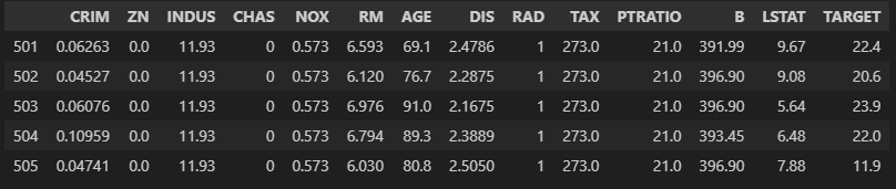
칼럼 선정
import torch
import torch.nn as nn
import torch.nn.functional as F
import torch.optim as optim
cols = ["TARGET", "INDUS", "RM", "LSTAT", "NOX", "DIS"]
data = torch.tensor(df[cols].values).float()
data.shape
-----------------------------------------------------------
torch.Size([506, 6])
특성과 라벨로 분리
x = data[:, 1:]
y = data[:, :1]

print(x.shape, y.shape)
--------------------------------
torch.Size([506, 5]) torch.Size([506, 1])
하이퍼파라미터
n_epochs = 2000
learning_rate = 1e-3
print_interval = 100
모델 학습
model = nn.Linear(x.size(-1), y.size(-1))

# SGD(stochastic gradient descent, 확률적 경사하강법)
optimizer = optim.SGD(model.parameters(), lr=learning_rate)

for i in range(n_epochs):
    y_hat = model(x)
    loss = F.mse_loss(y_hat, y)

    optimizer.zero_grad()   # optimizer 초기화
    loss.backward()     # 미분

    optimizer.step()    # 파라미터 업데이트

    if (i+1)%print_interval==0:
        print("Epoch %d: loss=%.4e" %(i+1, loss))
-----------------------------------------------------
Epoch 100: loss=4.4202e+01
Epoch 200: loss=3.7470e+01
...
Epoch 1900: loss=2.8987e+01
Epoch 2000: loss=2.8986e+01
모델 학습결과
df = pd.DataFrame(torch.cat([y, y_hat], dim=1).detach_().numpy(), columns=["y", "y_hat"])
sns.pairplot(df, height=5)
plt.show()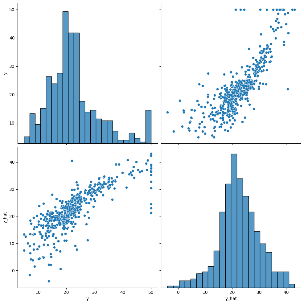
3. 유방암 예측
import pandas as pd
import seaborn as sns
import matplotlib.pyplot as plt
from sklearn.datasets import load_breast_cancer
cancer = load_breast_cancer()

# print(cancer.DESCR)
데이터 정리
df = pd.DataFrame(cancer.data, columns=cancer.feature_names)
df['class'] = cancer.target
df.tail()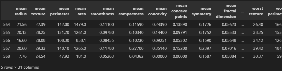
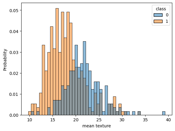
칼럼 선정
cols = ['mean radius', 'mean texture',
        'mean smoothness', 'mean compactness', 'mean concave points',
        'worst radius', 'worst texture',
         'worst smoothness', 'worst compactness', 'worst concave points',
         'class']

for c in cols[:-1]:
    sns.histplot(df, x=c, hue=cols[-1], bins=50, stat="probability")
    plt.show()	# 이미지 다수 생략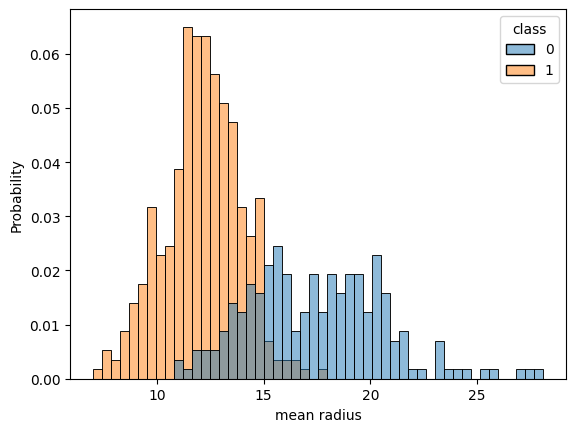
데이터 분리
data = torch.from_numpy(df[cols].values).float()

x = data[:, :-1]
y = data[:, -1:]

print(x.shape, y.shape)
-----------------------------------------------------
torch.Size([569, 10]) torch.Size([569, 1])
하이퍼파라미터
n_epochs = 200000
learning_rate = 1e-2
print_interval = 10000
모델링
class MyModel(nn.Module):
    def __init__(self, input_dim, output_dim):
        super(MyModel, self).__init__()
        self.input_dim, self.output_dim = input_dim, output_dim
        self.linear = nn.Linear(input_dim, output_dim)
        self.act = nn.Sigmoid()

    def forward(self, x):
        y = self.act(self.linear(x))

        return y
model = MyModel(input_dim=x.size(-1),
output_dim=y.size(-1))
crit = nn.BCELoss() # Binary Cross Entropy
optimizer = optim.SGD(model.parameters(), lr=learning_rate)모델 학습
for i in range(n_epochs):
    y_hat = model(x)
    loss = crit(y_hat, y)

    optimizer.zero_grad()
    loss.backward()

    optimizer.step()

    if (i+1)%print_interval==0:
        print(f"Epoch {i+1}: loss={loss.item():.4f}")
---------------------------------------------------------
Epoch 10000: loss=0.2796
Epoch 20000: loss=0.2299
...
Epoch 190000: loss=0.1167
Epoch 200000: loss=0.1156
모델 학습결과
correct_cnt = (y == (y_hat > .5)).sum()
total_cnt = float(y.size(0))

print("Accuracy: %.4f" %(correct_cnt/total_cnt))
---------------------------------------------------
Accuracy: 0.9649
df = pd.DataFrame(torch.cat([y, y_hat], dim=1).detach().numpy(), columns=["y", "y_hat"])
sns.histplot(df, x="y_hat", hue="y", bins=50, stat="probability")
plt.show()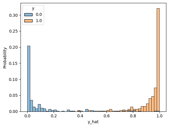
4. MNIST
import torch
import torch.nn as nn
import torch.nn.functional as F
import torch.optim as optim
from torchvision import datasets, transforms

import matplotlib.pyplot as plt
%matplotlib inline
Set Cuda
device = torch.device("cuda" if torch.cuda.is_available() else "cpu")
print("Current device is", device)
----------------------------------------------------------------------
Current device is cpu
Datasets Load
import os
# os.listdir("../data")
train_data = datasets.MNIST(root="../data",   # data save path
                            train=True,       # train data
                            download=True,    # download on
                            transform=transforms.ToTensor())

test_data = datasets.MNIST(root="../data",    # data save path
                            train=False,      # test data
                            transform=transforms.ToTensor())

print("number of training data: ", len(train_data))
print("number of test data: ", len(test_data))
-----------------------------------------------------------------
number of training data:  60000
number of test data:  10000
Data Check
image, label = train_data[0]
image.shape, image.squeeze().shape
# 첫번째 차원이 channel
------------------------------------------------
(torch.Size([1, 28, 28]), torch.Size([28, 28]))plt.imshow(image.squeeze().numpy(), cmap="gray")
plt.title("label : %s" %label)
plt.show()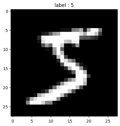
Mini batch configure
batch_size = 50
learning_rate = 0.0001
epoch_num = 15

train_loader = torch.utils.data.DataLoader(dataset = train_data,
                                           batch_size=batch_size,
                                           shuffle=True)

test_loader = torch.utils.data.DataLoader(dataset = test_data,
                                           batch_size=batch_size,
                                           shuffle=True)

first_batch = train_loader.__iter__().__next__()
print("{:15s} | {:<25s} | {}".format("name", "type", "size"))
print("{:15s} | {:<25s} | {}".format("Num of Batch", "", len(train_loader)))
print("{:15s} | {:<25s} | {}".format("first_batch", str(type(first_batch)), len(first_batch)))
print("{:15s} | {:<25s} | {}".format("first_batch[0]", str(type(first_batch[0])), first_batch[0].shape))
print("{:15s} | {:<25s} | {}".format("first_batch[1]", str(type(first_batch[1])), first_batch[1].shape))
-----------------------------------------------------------------------------------------------------------
name            | type                      | size
Num of Batch    |                           | 1200
first_batch     | <class 'list'>            | 2
first_batch[0]  | <class 'torch.Tensor'>    | torch.Size([50, 1, 28, 28])
first_batch[1]  | <class 'torch.Tensor'>    | torch.Size([50])
Modeling
- nn.Linear(3136, 1000)으로 설정되어 있다
- (28,28) -> MaxPooling2d 2번 -> (7,7) 여기에 channel_cnt를 곱함
- 하지만 연결계층의 입력크기는 일반적으로 특징을 잘 포착할 수 있을 만큼 크게 선택됨
- 입력크기 너무 크면 과적합, 작으면 정보를 모두 포착하지 못해서 올바른 학습불가
- 따라서 시행착오를 통해서 최적의 입력크기를 찾아야한다
class CNN(nn.Module):
    def __init__(self):
        super(CNN, self).__init__()
        self.conv1 = nn.Conv2d(1, 32, 3, 1, padding="same")
        self.conv2 = nn.Conv2d(32, 64, 3, 1, padding="same")
        self.dropout = nn.Dropout2d(0.25)

        self.fc1 = nn.Linear(3136, 1000)
        self.fc2 = nn.Linear(1000, 10)

    def forward(self, x):
        x = self.conv1(x)
        x = F.relu(x)
        x = F.max_pool2d(x,2)

        x = self.conv2(x)
        x = F.relu(x)
        x = F.max_pool2d(x,2)

        x = self.dropout(x)
        x = torch.flatten(x,1)

        x = self.fc1(x)
        x = F.relu(x)
        x = self.fc2(x)
        output = F.log_softmax(x, dim=1)

        return output
model = CNN().to(device)
optimizer = optim.Adam(model.parameters(), lr=learning_rate)
criterion = nn.CrossEntropyLoss()Model Learning
from time import time

model.train()
i = 1
for epoch in range(epoch_num):
    start_time_each_epoch = time()
    for data, target in train_loader:
        data = data.to(device)
        target = target.to(device)
        optimizer.zero_grad()
        output = model(data)
        loss = criterion(output, target)
        loss.backward()
        optimizer.step()
        if i%1000==0:
            print("Time: %.3f\tTrain Step: %d\tLoss: %.3f\t" %(time() - start_time_each_epoch, i, loss.item()))
        i+=1
---------------------------------------------------------------------------
Time: 81.436	Train Step: 1000	Loss: 0.191
Time: 69.932	Train Step: 2000	Loss: 0.033
Time: 53.119	Train Step: 3000	Loss: 0.014
Time: 52.150	Train Step: 4000	Loss: 0.132
Time: 22.078	Train Step: 5000	Loss: 0.192
Time: 136.500	Train Step: 6000	Loss: 0.178
Time: 114.181	Train Step: 7000	Loss: 0.048
Time: 90.783	Train Step: 8000	Loss: 0.018
Time: 68.979	Train Step: 9000	Loss: 0.020
Time: 43.789	Train Step: 10000	Loss: 0.005
Time: 20.056	Train Step: 11000	Loss: 0.055
Time: 97.013	Train Step: 12000	Loss: 0.000
Time: 78.883	Train Step: 13000	Loss: 0.027
Time: 62.891	Train Step: 14000	Loss: 0.005
Time: 47.510	Train Step: 15000	Loss: 0.003
Time: 31.382	Train Step: 16000	Loss: 0.000
Time: 15.918	Train Step: 17000	Loss: 0.001
Time: 95.073	Train Step: 18000	Loss: 0.018
Model Eval
model.eval()
correct = 0

for data, target in test_loader:
    data = data.to(device)
    target = target.to(device)
    output = model(data)
    prediction = output.data.max(1)[1]
    correct += prediction.eq(target.data).sum()

print("Test set: Accuracy: %.2f" %(100.*correct / len(test_loader.dataset)))
------------------------------------------------------------------------------
Test set: Accuracy: 99.08