Day 1

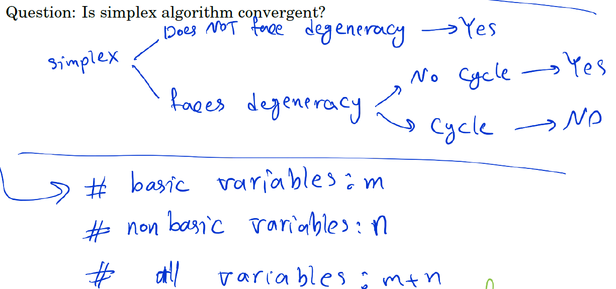
Degeneracy

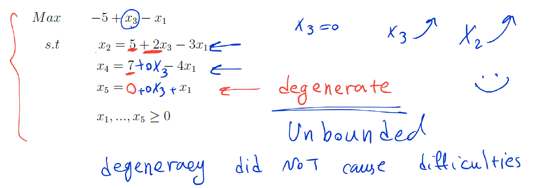
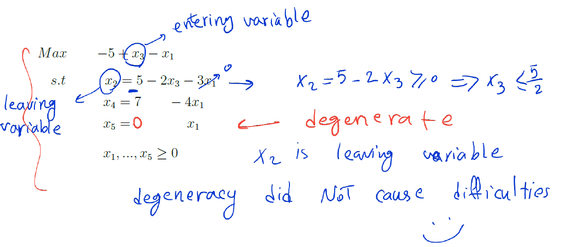
In the examples above the degeneracy is not cause any problem. However, problem arises when a degenerate dictionary produces degenerate pivots.

We say that a pivot is a degenerate pivot if one of the ratios in the calculations of the leaving variable is positive infinity:i.e., if the numerator is positive and the denominoator vanished.

Example

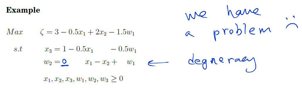
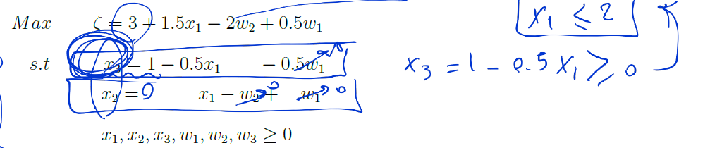
For this dictionary, the entering variable is x2 and the ratios computed to determine the leaving variable are 0 and positive infinity. Hence, the leaving variable is w2, and the fact taht the ratio is infinite means that as soon as x2 is increased from zero to a positive value, w2 will go negative. Therefore, x2 cannot really increase.

feasible solution: x1=0, x2=0, w1=0, w2=0, x3=1
basic variables: x3, w2
non-basic variables: x1, x2, w1
value of the objective function: 3
entering variable: x2
leaving variable: w2

As soon as x2 increases from zero to a positive value, w2 will go negative. Therefore, x2 remains zero. Let us look at the result of a degenerate pivot.

Note that value of the objective function remains unchanged at 3. Hence, this degenerate pivot has not produced any increase in the objective function value. Furthermore, the values of the variables have not even changed: both before and after this degenerate pivot, they are (x1, x2, x3, x4, x5) = (0, 0, 1, 0, 0)

feasible solution: x1=0, x2=0, w1=0, w2=0, x3=1
basic variables: x3, x2
non-basic variables: x1, w1, w2
value of the objective function: 3
entering variable: x1
leaving variable: x3

As we see after the degenerage pivoting that has been done, the feasible solution and the value of the objective function are the same, but the basic and nonbasic variables are different.

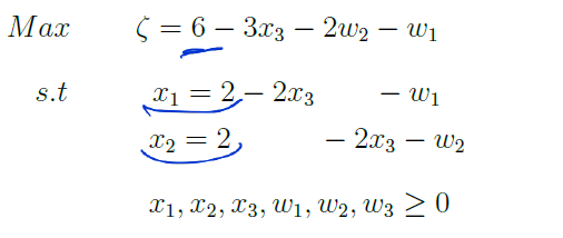
The next pivot is not a degenerate pivot because by increasing x3, x1 can be increased to 2 (Check the ratio)

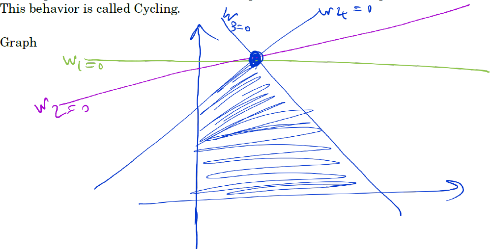
When one reaches a degenerate dictionary, it is usual that one or more of the subsequent pivots will be degenerate but that eventually a nondegenerate pivot will lead us away from these degenerate dictionaries. The real danger is taht the simplex method will make a subsequence of degenerate pivots and eventually return to a dictionary that has appeared before, in which case the simplex method enters an infinite lop and never finds an optimal solution. This behaviour is called cycling.

feasible (optimal) solution: x1=2, x2=2, x3=0, w1=0, w2=0
basic variables: x1, x2
non-basic variables: x3, w1, w2
(optimal) value fo the objective function: 6

In this example we were lucky. We faced degeneracy but eventually a nondegenerate pivot lead us away from degeneracy. However, sometimes after some degenerate pivots we return to dictionary that has happened before. In this case the simplex method enters an infinite loop and never find the optimal solution. This behaviot is called Cycling.

Unfortunately, under certain pivoting rules, cycling is possible.

• Choose the entering variable as the one with the largest coefficient in the objective function row of the dictionary.
• When two or more variables compete for leaving basis, pick an x-variable over a slack variable and , if there is a choice, use the variable with the smallest subscript. In other words, reading left to right, pick the first leaving variable candidate from the list:
  

Day 2

Degenearcy

As we did last time, the simplex method sometimes enters an infinite loop of degenerate pivots. Unfortunately cycling is possible even when usnig one of the most popular pivoting rules:

• Choose the entering variabels as the one with the largest coefficient in the objective function
• When two or more variables are candidate for leaving the basis, pick x-variable rather than the slack variable. If there is still a choice, use the variable with the smallest subscript
• order: x1, x2,... xn, w1, ..., wm

Example

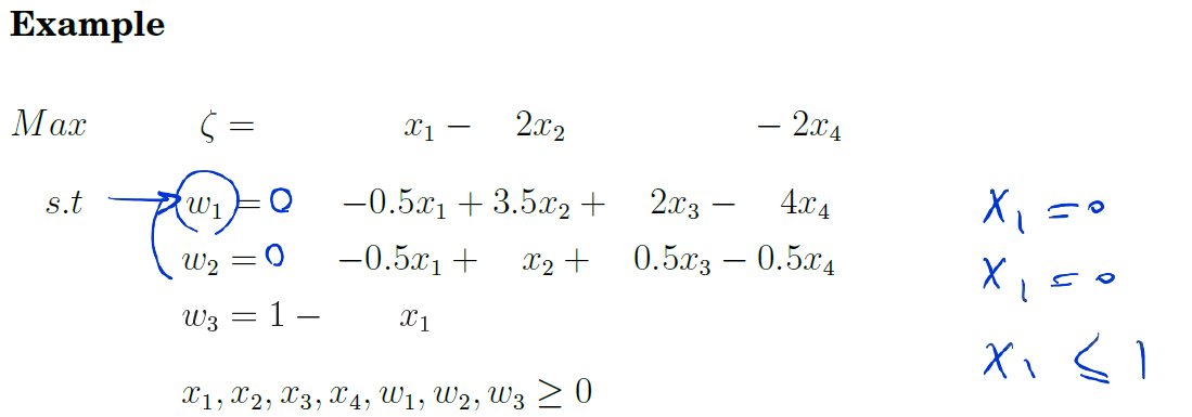
feasible solution: x1=0, x2=0, x3=0, x4=0, w1=0, w2=0, w3=1
basic variables: w1, w2, w3
non-basic variables: x1, x2, x3, x4
value of the objective function: 0
entering variable: x1
leaving variable: w1

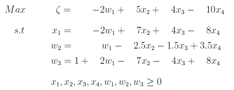
feasible solution: x1=0, x2=0, x3=0, x4=0, w1=0, w2=0, w3=1
basic variables: x1, w2, w3
non-basic variables: x2, x3, x4, w1
value of the objective function: 0
entering variable: x2
leaving variable:

We keep iterating again and again and again until
The sixth iteration of the simplex will generate:

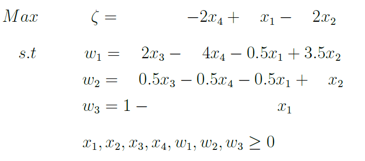
Note that we have come back to the original dictionary. From here on the simplex method cycles through these iterations and does not move towards the optimal solution.

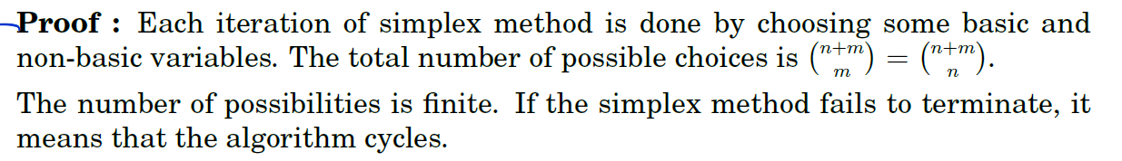
Theorem 3.1 If the simplex method fails to terminate, then it must cycle

Day 3

Degeneracy

Last time we saw that even by following the most popular pivoting rule, the simplex method might get into a cycle of degeneracy and not converge to the optimal solution.

Question: Are there pivoting rules for which the simplex method, for sure, converges? Answer: Yes. We are going to present two pivoting rules.

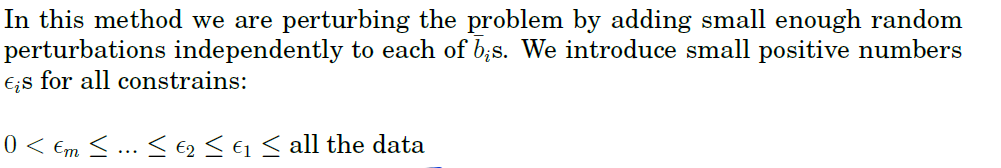
The Perturbation/Lexicographic Method

The first method is based on the observation that degeneracy is sort of an accident. That is, a dictionary is degenerate if one or more of the bi's vanishe. Out examples have generally used small integers for the data, and in this case it does not seem too surprising that sometimes cancellations occur and we end up with a degenerate dictionary. But each right-hand side could in fact be any real number, and in the world of real numbers the occurence of any specific number, such as zero, seems to be quite unlikely. So how about perturbing a given problem by adding small random perturbations independently to each of the right-hand sides? If these perturbations are small enough, we can think of them as insignificant and hence not really chaning the problem. If they are chosen independently, then the probability of an exact cancellation is zero.

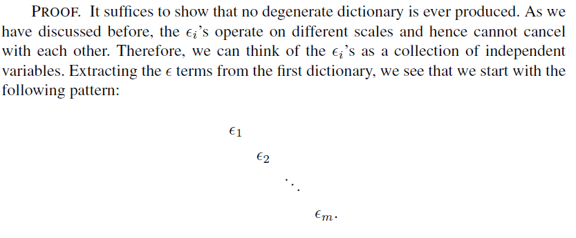
What we mean by this is that no linaer combinations of the epsilons using coefficients that might arise int he course of the simplex method can ever produce a number whose size is of the same order as the data in the problem.

Consider the following degenerate dictionary:

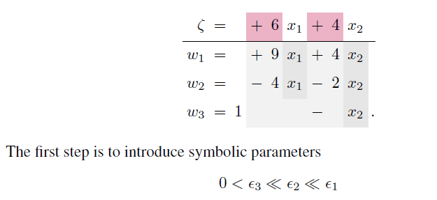
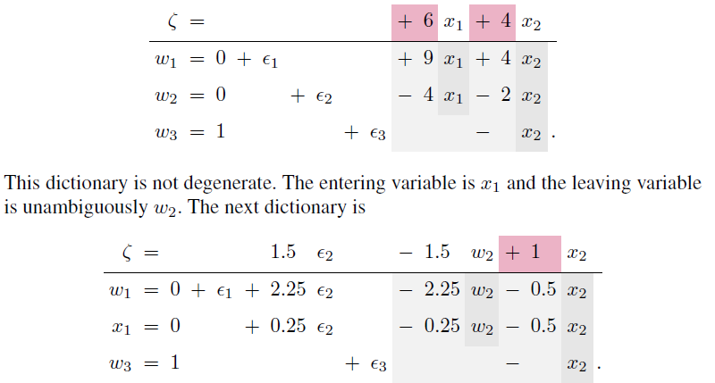
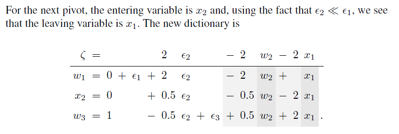
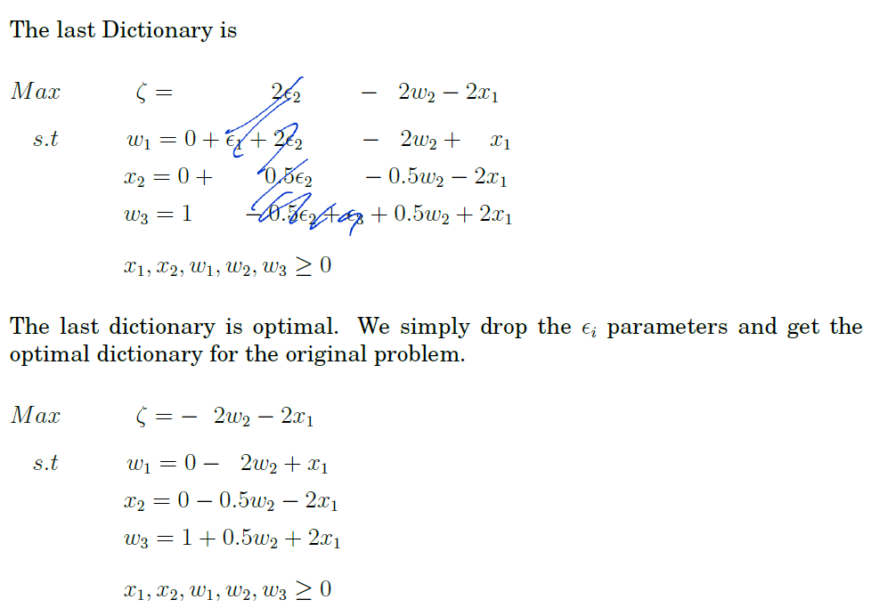
When treating the epsilons as symbols, the method is called the lexicographic method. Note that the lexicographic method does not affect the choice of entering variable but does amount to a precise prescription for the choice of leaving variable. It turns out that lexicographic method produces a variant of the simplex method that never cycles.

Theorem 3.2 The simplex method always terminates provided that the leaving variable is selected by the lexicographic method.

Bland's Rule

Both the entering and leaving variable should be selected from their respective sets of choices by choosing the variable xk with the smallest index k.

Theorem 3.3 The simplex method always terminates provided that both the entering and leaving variable are chosen according to Bland's rule.

Fundamental Theorem of Linear Programming

Now that we have a phase I algorithm and a variant of the simplex method that is guaranteed to terminate, we can summarize the main point of this chapter in the following theorem.

Theorem 3.4 For an arbitrary linear programming in standard form, the following statements are true.

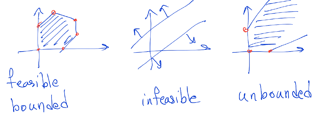
• If there is no optimal solution, then the problem is either infeasible or unbounded.
• If a feasible solution exists, then a basic feasible solution exists.
• If an optimal solution exists, then a basic optimal solution exists.

Proof The Phase I algorithm either proves that the problem is infeasible or produces a basic feasible solution. The phase II algorithm either discovers that the problem is unbounded or finds a basic optimal solution. (These statements depend on using a variant of the simplex method does not cycle which we know to exist)

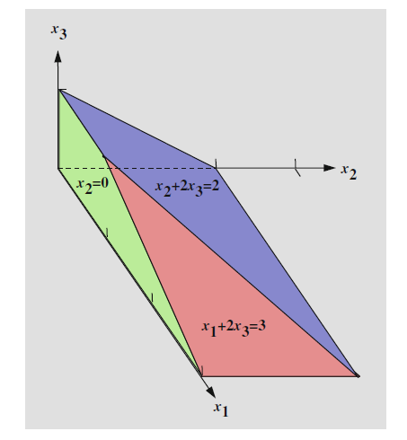
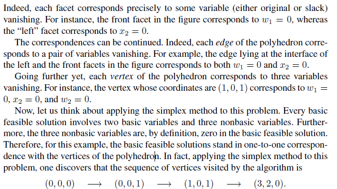
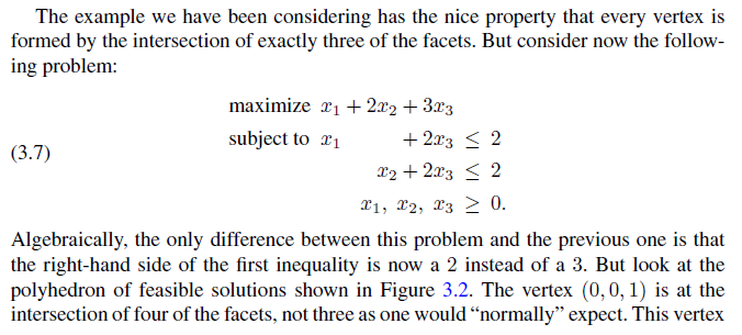
geometry

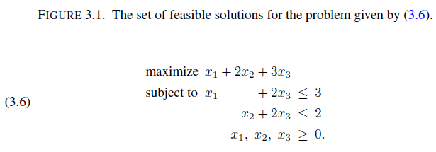
As we saw in the previous chapter, the set of feasible solutions for a problem in two dimensions is the intersection of a number of half-planes, i.e., a polygon. In three dimensions, the situation si similar. Consider, for example, the following problem:

leaving variable 정하는 규칙?
영향을 바든ㄴ 것 중 가장 작은 boundary를 가지는 것?