
「권철민(2020).파이썬 머신러닝 완벽가이드(개정판).위키북스」 책으로 공부한 뒤 정리한 내용.
1. 사이킷런
Scikit-learn (formerly scikits.learn and also known as sklearn) is a free software machine learning library for the Python programming language. It features various classification, regression and clustering algorithms including support vector machines, random forests, gradient boosting, k-means and DBSCAN, and is designed to interoperate with the Python numerical and scientific libraries NumPy and SciPy.(위키백과)
사이킷런은 파이썬 머신러닝 라이브러리 중 가장 많이 사용되며, 파이썬 기반의 다른 머신러닝 패키지도 사이킷런 스타일의 API를 지향한다.
2. 사이킷런의 기반 프레임워크
(1) 지도학습
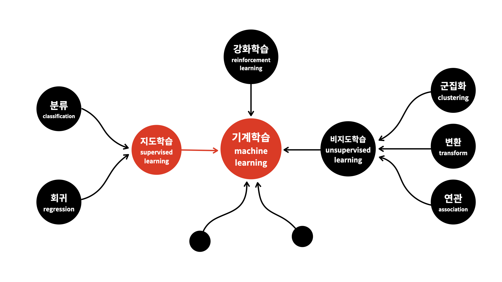
이미지 출처: 오픈튜토리얼스 생활코딩
지도학습은 훈련 데이터로부터 함수를 유추해내기 위한 기계학습 방법 중 하나이다. 훈련 데이터를 통해 유추된 함수 중 연속적인 값을 출력하는 것을 회귀라 하고, 주어진 입력 벡터가 어떤 종류인지를 표식하는 것을 분류라고 한다.
(2) Estimator
사이킷런은 머신러닝 모델 학습을 위해 fit()을, 학습된 모델의 예측을 위해 predict() 메소드를 제공한다. 지도학습의 주요한 두 축인 분류와 회귀의 다양한 알고리즘을 구현한 사이킷런 클래스는 이 두 메소드만을 이용해 학습과 예측 결과를 반환한다. 사이킷런에서 분류 알고리즘을 구현한 클래스를 Classifier로, 회귀 알고리즘을 구현한 클래스를 Regressor라고 칭하며, 이 둘을 합쳐 Estimator라고 부른다.
3. 사이킷런의 내장 데이터세트
sklearn.datasets에는 예제로 활용 가능한 데이터 세트들이 내장되어있다.
>>> from sklearn.datasets import load_iris사이킷런에 내장된 데이터 세트는 일반적으로 딕셔너리 형태로 되어있다. 딕셔너리의 키는 보통 data, target, target_name, feature_names, DESCR로 구성되어있다.
🤖data: 피쳐의 데이터 세트(ndarray)
🤖target: 분류 시에는 레이블 값, 회귀 시에는 결괏값 데이터 세트 (ndarray)
🤖target_names: 개별 레이블 이름(list)
🤖feature_names: 피쳐의 이름(list)
🤖DESCR: 데이터 세트와 각 피쳐에 대한 설명(str)
>>> iris_data = load_iris()
>>> type(iris_data)
<class 'sklearn.utils.Bunch'>
>>> iris_data.keys()
dict_keys(['data', 'target', 'frame', 'target_names', 'DESCR', 'feature_names', 'filename'])
>>> iris_data['data']
array([[5.1, 3.5, 1.4, 0.2],
       [4.9, 3. , 1.4, 0.2],
       [4.7, 3.2, 1.3, 0.2],
     	(중략)
       [6.5, 3. , 5.2, 2. ],
       [6.2, 3.4, 5.4, 2.3],
       [5.9, 3. , 5.1, 1.8]])
>>> iris_data['target']
array([0, 0, 0, 0, 0, 0, 0, 0, 0, 0, 0, 0, 0, 0, 0, 0, 0, 0, 0, 0, 0, 0,
       0, 0, 0, 0, 0, 0, 0, 0, 0, 0, 0, 0, 0, 0, 0, 0, 0, 0, 0, 0, 0, 0,
       0, 0, 0, 0, 0, 0, 1, 1, 1, 1, 1, 1, 1, 1, 1, 1, 1, 1, 1, 1, 1, 1,
       1, 1, 1, 1, 1, 1, 1, 1, 1, 1, 1, 1, 1, 1, 1, 1, 1, 1, 1, 1, 1, 1,
       1, 1, 1, 1, 1, 1, 1, 1, 1, 1, 1, 1, 2, 2, 2, 2, 2, 2, 2, 2, 2, 2,
       2, 2, 2, 2, 2, 2, 2, 2, 2, 2, 2, 2, 2, 2, 2, 2, 2, 2, 2, 2, 2, 2,
       2, 2, 2, 2, 2, 2, 2, 2, 2, 2, 2, 2, 2, 2, 2, 2, 2, 2])
>>> iris_data['target_names']
array(['setosa', 'versicolor', 'virginica'], dtype='<U10')
>>> iris_data['feature_names']
['sepal length (cm)', 'sepal width (cm)', 'petal length (cm)', 'petal width (cm)']
여기서 target의 값이 0이면 'setosa', 1이면 'versicolor', 2이면 'virginica'이다.
4. Model Selection 모듈
(1) train_test_split()
Decision Trees (DTs) are a non-parametric supervised learning method used for classification and regression. The goal is to create a model that predicts the value of a target variable by learning simple decision rules inferred from the data features. A tree can be seen as a piecewise constant approximation.
>>> import sklearn
>>> from sklearn.datasets import load_iris
>>> from sklearn.tree import DecisionTreeClassifier()
>>> from sklearn.metrics import accuracy_score
>>> iris = load_iris()
>>> dt_clf = DecisionTreeClassifier
>>> train_data = iris.data
>>> train_label = iris.target
>>> dt_clf.fit(train_data, train_label)
DecisionTreeClassifier()
>>> pred = dt_clf.predict(train_data)
>>> accuracy_score(train_label, pred)
1.0
학습 데이터 세트와 테스트 데이터 세트를 분리하지 않으면 예측 정확도가 1.0이 나온다. 이는 이미 학습한 데이터 세트를 기반으로 예측했기 때문이다. 학습을 수행하기 전 테스트용 데이터 세트를 분리하여야 유의미한 정확도 테스트를 할 수 있다.
>>> from sklearn.model_selection import train_test_split
>>> X_train, X_test, y_train, y_test = train_test_split(iris.data, iris.target, test_size=0.3, random_state=121)
>>> dt_clf.fit(X_train, y_train)
DecisionTreeClassifier()
>>> pred = dt_clf.predict(X_test)
>>> accuracy_score(y_test, pred)
0.9555555555555556
학습용 피처 데이터 세트와 테스트용 피처 데이터 세트를 각각 X_train과 X_test로, 학습용 레이블 데이터 세트와 테스트용 레이블 데이터 세트를 각각 y_train과 y_test로 반환하였다.
test size를 0.3으로 지정하였기 때문에, 전체 데이터 중 30%가 테스트 데이터, 70%가 학습 데이터로 배정되었다. train_test_split()의 파라미터는 다음과 같다.
train_test_split(*arrays, test_size=None, train_size=None, random_state=None, shuffle=True, stratify=None)
첫번째 array들에는 피처 데이터 세트(iris.data)와 레이블 데이터 세트(iris.target)이 들어갔다. random_state는 호출할 때마다 같은 학습/테스트 용 데이터 세트를 생성하기 위해 주어지는 난수 발생 값이다.
이렇게 테스트용 데이터 세트와 학습용 데이터 세트를 분리하자 정확도가 약 95.56%로 측정되었다.
(2) 교차 검증
테스트 데이터 세트와 학습용 데이터 세트를 분리함으로써 머신러닝 알고리즘의 예측 성능을 평가할 수 있다. 하지만 이 방법은 과적합에 취약하다. 즉, 모델이 학습 데이터에만 최적화되어, 다른 데이터로 실제 예측을 수행하는 경우에는 성능이 떨어질 수 있다. 이를 방지하기 위하여 교차 검증을 이용한다.
K 폴드 교차 검증
K 폴드 교차 검증은 가장 보편적으로 사용되는 교차 검증 기법으로, K개의 데이터 폴드 세트를 만들어서 K번만큼 각 폴드 세트에 학습과 검증 평가를 반복적으로 수행하는 작업이다.
>>> import sklearn
>>> from sklearn.tree import DecisionTreeClassifier
>>> from sklearn.metrics import accuracy_score
>>> from sklearn.model_selection import KFold
>>> import numpy as np
>>> from sklearn.datasets import load_iris
>>> iris = load_iris()
>>> features = iris.data
>>> label = iris.target
>>> dt_clf = DecisionTreeClassifier(random_state=156)
>>> kfold = KFold(n_splits=5)
>>> cv_accuracy = []
>>> features.shape[0]
150
총 데이터 세트의 크기는 150이며, 폴드 데이터 세트는 5개로 지정하였다. 데이터 세트를 30개씩 나눈 뒤 4개의 세트는 학습용, 1개의 세트는 테스트용으로 사용하며, 이 과정을 5번 반복한다.
>>> n = 0
>>> for train_index, test_index in kfold.split(features):
...     X_train, X_test = features[train_index], features[test_index]
...     y_train, y_test = label[train_index], label[test_index]
...     dt_clf.fit(X_train, y_train)
...     pred = dt_clf.predict(X_test)
...     n += 1
...     accuracy = np.round(accuracy_score(y_test, pred),4)
...     cv_accuracy.append(accuracy)
...
DecisionTreeClassifier(random_state=156)
DecisionTreeClassifier(random_state=156)
DecisionTreeClassifier(random_state=156)
DecisionTreeClassifier(random_state=156)
DecisionTreeClassifier(random_state=156)
>>> np.mean(cv_accuracy)
0.9
Stratified K 폴드
Stratified K 폴드는 불균형한 분포도를 가진 레이블 데이터 집합을 위한 K 폴드 방식으로, 원본 데이터 집합의 레이블 분포를 먼저 고려한 뒤 이 분포와 동일하게 학습과 검증 데이터 세트를 분배한다. 일반적으로 분류에서의 교차검증에는 Stratified K 폴드를 사용해야하지만, 회귀에서는 동 방식이 지원되지 않는다. 회귀의 결정값은 연속된 숫자값이기 때문에 결정값별로 분포를 정하는 의미가 없기 때문이다.
cross_val_score()
cross_val_score()은 폴드 세트를 설정하고, for 루프를 돌며 학습 및 테스트 데이터의 인덱스를 추출한 뒤, 반복적으로 학습과 예측을 수행하고 예측 성능을 반환하는 과정을 한꺼번에 수행한다. cross_val_score()의 형태는 다음과 같다
cross_val_score(estimator, X, y=None, , groups=None, scoring=None, cv=None, n_jobs=None, verbose=0, fit_params=None, pre_dispatch='2n_jobs', error_score=nan)
>>> from sklearn.model_selection import cross_val_score, cross_validate
>>>
>>> scores = cross_val_score(dt_clf, features, label, scoring='accuracy', cv=3)
>>> np.round(scores,4)
array([0.98, 0.94, 0.98])
>>> np.round(np.mean(scores),4)
0.9667
cross_val_score()을 사용하면 분류의 경우 StraifiedKFold를, 회귀의 경우 KFold를 자동적으로 사용한다.
