[빅 리더 AI] 머신러닝 1~4일차

빅데이터 분석 절차
1. 기획 (위험성 분석)
2. 데이터 수집
3. 데이터 전처리
4. 모델 선택
5. 평가 및 적용

위험성 분석

• 예측에 실패했을 때의 위험성을 그 분야 전문가와 논의하는 것

모델의 정확도

• 보통 95% 이상이면 상용화할만 하다고 판단함

Titanic

데이터 확인

import pandas as pd
import numpy as np
import matplotlib.pyplot as plt
import seaborn as sns

df = sns.load_dataset('titanic') # seaborn에 유명한 데이터셋 몇 개가 이미 올라와 있다
df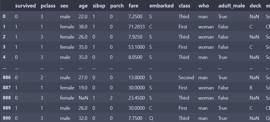

df.shape

(891, 15)

df.pclass.value_counts()

3    491
1    216
2    184
Name: pclass, dtype: int64

df.info()

<class 'pandas.core.frame.DataFrame'>
RangeIndex: 891 entries, 0 to 890
Data columns (total 15 columns):
 #   Column       Non-Null Count  Dtype   
---  ------       --------------  -----   
 0   survived     891 non-null    int64   
 1   pclass       891 non-null    int64   
 2   sex          891 non-null    object  
 3   age          714 non-null    float64 
 4   sibsp        891 non-null    int64   
 5   parch        891 non-null    int64   
 6   fare         891 non-null    float64 
 7   embarked     889 non-null    object  
 8   class        891 non-null    category
 9   who          891 non-null    object  
 10  adult_male   891 non-null    bool    
 11  deck         203 non-null    category
 12  embark_town  889 non-null    object  
 13  alive        891 non-null    object  
 14  alone        891 non-null    bool    
dtypes: bool(2), category(2), float64(2), int64(4), object(5)
memory usage: 80.7+ KB

for i in df.columns:
    print('feature: ',i)
    print(df[i].value_counts())
    plt.figure(figsize=(20,10))
    df[i].value_counts().plot(kind='bar')
    plt.show()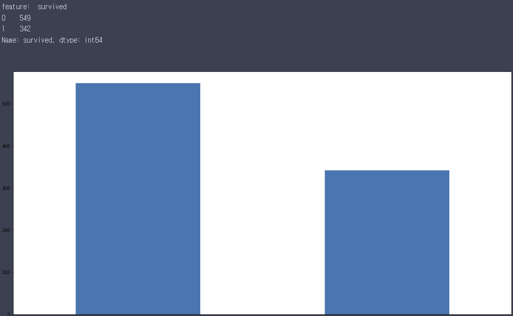

df.age.plot(kind='hist', bins=40)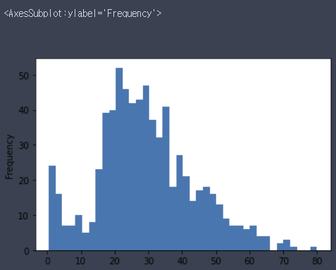

df.describe() # include='all' 옵션을 주면 숫자형이 아닌 컬럼도 나온다.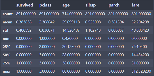

결측치 처리

print('피쳐별 결측치: \n',df.isna().sum())
print('전체 결측치 수: ', df.isna().sum().sum())

피쳐별 결측치: 
 survived         0
pclass           0
sex              0
age            177
sibsp            0
parch            0
fare             0
embarked         2
class            0
who              0
adult_male       0
deck           688
embark_town      2
alive            0
alone            0
dtype: int64
전체 결측치 수:  869

df.embark_town.value_counts().plot(kind='bar')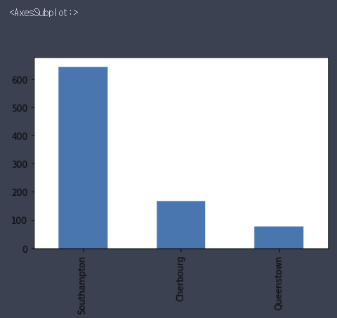

df.drop('embark_town', axis=1, inplace=True)
df.embarked.fillna('S', inplace=True) # S가 대부분이기 때문에 2개의 결측치를 S로 채움
grouped = df.groupby(['sex','pclass'])
df_sp_grouped = grouped.age.median().unstack()
df_sp_grouped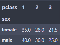

m1_md = df_sp_grouped.iloc[0, 0]
f1_md = df_sp_grouped.iloc[0, 1]
m2_md = df_sp_grouped.iloc[0, 2]
f2_md = df_sp_grouped.iloc[1, 0]
m3_md = df_sp_grouped.iloc[1, 1]
f3_md = df_sp_grouped.iloc[1, 2]

# pandas는 isna 조건을 내부로 넣는 것을 권장
df.loc[(df.sex=='male') & (df.pclass==1) & (df.age.isna()), 'age'] = m1_md
df.loc[(df.sex=='female') & (df.pclass==1) & (df.age.isna()), 'age'] = f1_md
df.loc[(df.sex=='male') & (df.pclass==2) & (df.age.isna()), 'age'] = m2_md
df.loc[(df.sex=='female') & (df.pclass==2) & (df.age.isna()), 'age'] = f2_md
df.loc[(df.sex=='male') & (df.pclass==3) & (df.age.isna()), 'age'] = m3_md
df.loc[(df.sex=='female') & (df.pclass==3) & (df.age.isna()), 'age'] = f3_md

# deck은 77%정도가 결측치라서 삭제로 결정
df.drop(columns='deck', inplace=True)
df.isna().sum().sum()

0

결측치 제거 추가 연습

df1 = sns.load_dataset('titanic')

# 1. embark_town 제거
df1.drop(columns='embark_town', inplace=True)

# 2. age열은 평균으로 결측치 업데이트
df1.age.fillna(df.age.mean(), inplace=True)

# 3. embarked, deck은 'N'으로 업데이트
df1.embarked.fillna('N', inplace=True)

df1.deck = df1.deck.astype('object') # deck의 type이 category 라서 새로운 category인 N으로 업데이트할 수 없어서 type을 object로 변형한다

df1.deck.fillna('N', inplace=True)

데이터 뜯어보기

df.corr() # 상관계수, 숫자형 데이터만 나옴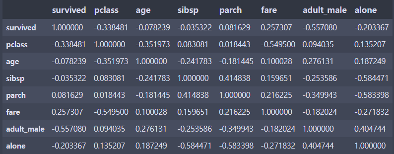

sns.heatmap(df.corr(), cmap='coolwarm', annot=True, cbar=True) 
# annot=True 옵션은 칸 안에 숫자를 표시한다
# cmap='coolwarm' 옵션을 주면 음수는 파란색, 양수는 빨간색 계열로 나온다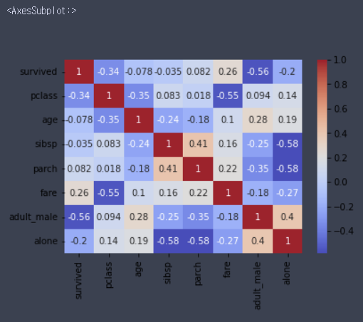

가정

• pclass와 생존여부의 상관관계가 높게 나타남
• 그럼 클래스에 따라 갑판과 멀리있는 룸에 투숙한 승객은 사망할 확률이 높음
• 그럼 신체적으로 뛰어난 사람이 더 생존확률이 높을 것
• 그럼 성인 남성의 생존률이 높을 것
• pclass와 생존여부, 성별과 생존여부, pclass와 성별과 생존여부를 살펴볼 필요가 있음

# pclass와 생존여부를 따로 보자
pd.crosstab(df.pclass, df.survived, margins=True) # margins=True 옵션을 주면 각 행, 열 별 합이 표시된다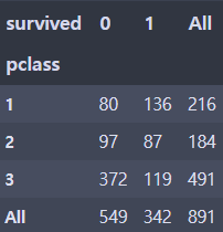

pd.crosstab(df.pclass, df.survived).plot(kind='bar')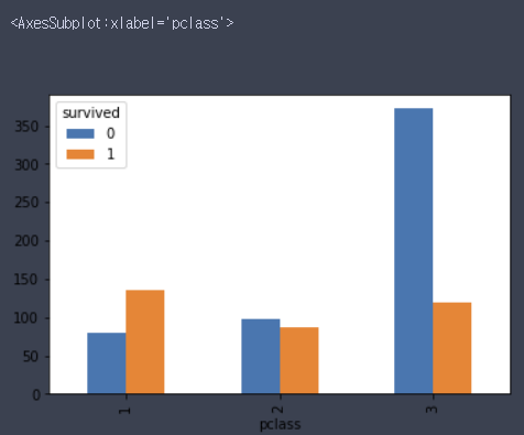

# 성별과 생존 여부
pd.crosstab(df.sex, df.survived, margins=True)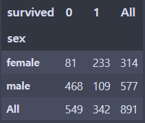

pd.crosstab(df.sex, df.survived).plot(kind='bar')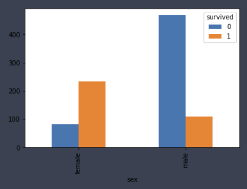

# pclass, 성별과 생존 여부
pd.crosstab([df.pclass, df.sex], df.survived, margins=True)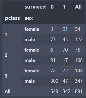

sns.violinplot(x='pclass', y='age', hue='survived', data=df, inner='quartile', split=True) # boxplot의 변형
# inner='quartile' 옵션은 분위수별로 선을 표시해준다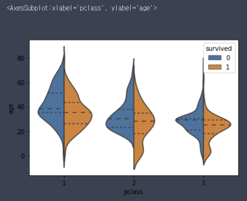

인코딩

• Label Encoding
  - Unique 값들을 오름차순 정렬을 시키고 먼저 나온 값에 낮은 정수를 부여
• One-Hot Encoding
  - 분류에서는 굳이 안해도 괜찮으나 회귀분석에서는 반드시 필요

Label Encoding

from sklearn.preprocessing import LabelEncoder

# df.dtypes[(df.dtypes=='object') | (df.dtypes=='bool') | (df.dtypes=='category')]
column_list = ['sex', 'embarked','class','who','adult_male','alive','alone']

for i in column_list:
    encoder = LabelEncoder()
    encoder.fit(df[i])
    df[i] = encoder.transform(df[i])
    
column_list2 = ['sex','embarked','class','who','adult_male','deck','alive','alone']
for i in column_list2:
    encoder = LabelEncoder()
    encoder.fit(df1[i])
    df1[i] = encoder.transform(df1[i])

데이터 전처리의 3단계

• 결측치 처리
• 인코딩
• feature scaling
  - 표준화: 데이터 분포를 정규분포로
  • 정규화

def standard_deviation(x):
    return (x - x.mean()) / x.std()
    
def normalization(x):
    return (x - x.min()) / (x.max() - x.min())

alive와 class 삭제

• x 값들 간에 80%를 넘어가는 상관관계가 있다는 것은 서로 독립적이지 않다는 것이라서 문제가 된다
• 나이는 연속적인 데이터이기 때문에 상관관계가 낮게 나옴

plt.figure(figsize=(10,10))
sns.heatmap(df.corr(), annot=True, cmap='coolwarm', cbar=False)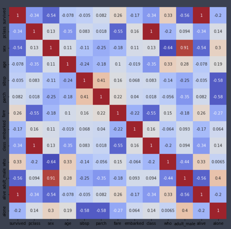

df.drop(['alive','class'], axis=1, inplace=True)
df1.drop(['alive','class'], axis=1, inplace=True)

데이터 분리

X = df.drop('survived',axis=1)
y = df.survived
X1 = df1.drop('survived', axis=1)
y1 = df1.survived

from sklearn.model_selection import train_test_split

X_train, X_test, y_train, y_test = train_test_split(X, y, test_size=0.2, random_state=42)

학습

from sklearn.tree import DecisionTreeClassifier
from sklearn.ensemble import RandomForestClassifier
from sklearn.linear_model import LogisticRegression
from sklearn.metrics import accuracy_score

dt_clf = DecisionTreeClassifier()
rf_clf = RandomForestClassifier(n_jobs=2) # n_jobs는 CPU의 코어를 몇개 사용할지 결정, -1은 전체 사용
lr_clf = LogisticRegression(n_jobs=2)

dt_clf.fit(X_train, y_train)
dt_pred = dt_clf.predict(X_test)
print('DecisionTree accuracy score: %.2f' %accuracy_score(y_test, dt_pred))

rf_clf.fit(X_train, y_train)
rf_pred = rf_clf.predict(X_test)
print('RandomForest accuracy score: %.2f' %accuracy_score(y_test, rf_pred))

lr_clf.fit(X_train, y_train)
lr_pred = lr_clf.predict(X_test)
print('LogisticRegression accuracy score: %.2f' %accuracy_score(y_test, lr_pred))

DecisionTree accuracy score: 0.77
RandomForest accuracy score: 0.82
LogisticRegression accuracy score: 0.80

K-Fold

from sklearn.model_selection import KFold

kfold = KFold(n_splits=5)

model_list = [dt_clf, rf_clf, lr_clf]
model_name_list = ['DecisionTree Classifier','RandomForest Classifier','LogisticRegression Classifier']

for j, val in enumerate(model_name_list):
    scores = []
    for i, (train, test) in enumerate(kfold.split(X)):
        X_train = X.values[train]
        X_test = X.values[test]
        y_train = y.values[train]
        y_test = y.values[test]

        model_list[j].fit(X_train, y_train)
        pred = model_list[j].predict(X_test)
        print('%s accuracy score: %.2f' %(model_name_list[j], accuracy_score(y_test, pred)))
        scores.append(accuracy_score(y_test, pred))
    print('kfold %s 평균 정확도: %.2f' %(model_name_list[j], np.mean(scores)))

DecisionTree Classifier accuracy score: 0.78
DecisionTree Classifier accuracy score: 0.79
DecisionTree Classifier accuracy score: 0.83
DecisionTree Classifier accuracy score: 0.78
DecisionTree Classifier accuracy score: 0.74
kfold DecisionTree Classifier 평균 정확도: 0.78
RandomForest Classifier accuracy score: 0.78
RandomForest Classifier accuracy score: 0.82
RandomForest Classifier accuracy score: 0.85
RandomForest Classifier accuracy score: 0.78
RandomForest Classifier accuracy score: 0.84
kfold RandomForest Classifier 평균 정확도: 0.81
LogisticRegression Classifier accuracy score: 0.82
LogisticRegression Classifier accuracy score: 0.81
LogisticRegression Classifier accuracy score: 0.79
LogisticRegression Classifier accuracy score: 0.78
LogisticRegression Classifier accuracy score: 0.88
kfold LogisticRegression Classifier 평균 정확도: 0.81

Stratified K-Fold

• positive:negative ratio 유지

from sklearn.model_selection import StratifiedKFold
skfold = StratifiedKFold()

model_list = [dt_clf, rf_clf, lr_clf]
model_name_list = ['DecisionTree Classifier','RandomForest Classifier','LogisticRegression Classifier']

for j, val in enumerate(model_name_list):
    scores = []
    for i, (train, test) in enumerate(skfold.split(X, y)):
        X_train = X.values[train]
        X_test = X.values[test]
        y_train = y.values[train]
        y_test = y.values[test]

        model_list[j].fit(X_train, y_train)
        pred = model_list[j].predict(X_test)
        print('%s accuracy score: %.2f' %(model_name_list[j], accuracy_score(y_test, pred)))
        scores.append(accuracy_score(y_test, pred))
    print('Stratifiedkfold %s 평균 정확도: %.2f' %(model_name_list[j], np.mean(scores)))

DecisionTree Classifier accuracy score: 0.79
DecisionTree Classifier accuracy score: 0.79
DecisionTree Classifier accuracy score: 0.83
DecisionTree Classifier accuracy score: 0.78
DecisionTree Classifier accuracy score: 0.78
Stratifiedkfold DecisionTree Classifier 평균 정확도: 0.79
RandomForest Classifier accuracy score: 0.79
RandomForest Classifier accuracy score: 0.80
RandomForest Classifier accuracy score: 0.85
RandomForest Classifier accuracy score: 0.78
RandomForest Classifier accuracy score: 0.83
Stratifiedkfold RandomForest Classifier 평균 정확도: 0.81
LogisticRegression Classifier accuracy score: 0.82
LogisticRegression Classifier accuracy score: 0.81
LogisticRegression Classifier accuracy score: 0.80
LogisticRegression Classifier accuracy score: 0.80
LogisticRegression Classifier accuracy score: 0.86
Stratifiedkfold LogisticRegression Classifier 평균 정확도: 0.82

K-Fold와 Stratified K-Fold

• 회귀 분석은 연속된 값이어서 비율을 맞춰서 나눌 수 없어 Stratified K-Fold를 사용할 수 없어 K-Fold를 쓸 수 밖에 없다

cross_val_score

from sklearn.model_selection import cross_val_score

cvs = cross_val_score(dt_clf, X, y, cv=5)
np.mean(cvs)

0.7867553825874082

cvs1 = cross_val_score(dt_clf, X1, y1, cv=5)
np.mean(cvs1)

0.7912748728893353

for model in model_list:
    cvs = cross_val_score(model, X, y, cv=5)
    cvs1 = cross_val_score(model, X1, y1, cv=5)
    print('cvs:',np.mean(cvs))
    print('cvs1:', np.mean(cvs1))

cvs: 0.7901387232439896
cvs1: 0.7957629778419434
cvs: 0.8069801016885318
cvs1: 0.8092210156299039
cvs: 0.8181783943255289
cvs1: 0.817048521750047

첨언

• 결측치 처리에 더 노력한 df와 그냥 단순하게 처리한 df1로 학습시킨 정확도가 비슷한 것을 확인 가능
• 결측치를 정확히 찾을 수 있는 경우라면 찾아서 넣으면 좋지만 처음에는 그냥 단순하게 처리하고 머신러닝을 돌리는 쪽이 나을 수 있다
• 시간이 남고 성능이 더 좋아지지 않을 것 같을 때 돌아와서 결측치를 조금 더 손보는 것이 합리적이다

하이퍼 파라미터 튜닝

X_train, X_test, y_train, y_test = train_test_split(X, y, test_size=0.1)
X_train_1, X_val, y_train_1, y_val = train_test_split(X_train, y_train, test_size=0.2)

from sklearn.model_selection import GridSearchCV

param_grid = {'max_depth':[2, 4, 5],
              'min_samples_split':[2, 4, 6],
              'min_samples_leaf':[1, 3, 5]}
              
dt_clf = DecisionTreeClassifier()
grid_dtclf = GridSearchCV(dt_clf, param_grid=param_grid, scoring='accuracy', n_jobs=-1, cv=5)

import time
start_time = time.time()
grid_dtclf.fit(X_train, y_train)
print('걸린 시간: ', time.time() - start_time)

걸린 시간:  2.61286997795105

grid_dtclf.best_params_

{'max_depth': 5, 'min_samples_leaf': 1, 'min_samples_split': 6}

grid_dtclf.best_score_

0.8302018633540372

best_dtclf = grid_dtclf.best_estimator_
best_pred = best_dtclf.predict(X_test)

lr_clf.get_params()

{'C': 1.0,
 'class_weight': None,
 'dual': False,
 'fit_intercept': True,
 'intercept_scaling': 1,
 'l1_ratio': None,
 'max_iter': 100,
 'multi_class': 'auto',
 'n_jobs': 2,
 'penalty': 'l2',
 'random_state': None,
 'solver': 'lbfgs',
 'tol': 0.0001,
 'verbose': 0,
 'warm_start': False}

회귀 성능 평가 지표

• MAE
• MSE
• RMSE
• R square

분류 성능 평가 지표

• 정확도
• 오차행렬
• 정밀도 & 재현율
• F1 스코어
• ROC AUC

Confusion Matrix

• 찾고자 하는 값을 양성으로 두는 것이 관례

from sklearn.metrics import confusion_matrix

confusion_matrix(y_test, best_pred)

array([[49,  9],
       [ 5, 27]], dtype=int64)

정밀도(Precision) & 재현율(Recall)

• 정밀도
  - 양성이라고 예측한 모든 경우에서 실제 양성인 경우
  • 실제 음성인 데이터 예측을 양성으로 잘못 판단(FP) 시 업무상 큰 영향이 발생하는 경우에 중요
  • 스팸 메일 판단
• 재현율
  - 실제 양성인 모든 경우에서 양성이라고 예측한 경우
  • 실제 양성 데이터를 음성이라고 잘못 판단(FN) 시 업무상 큰 영향이 발생하는 경우에 중요
  • 암 판단 모델, 금융 사기 모델

from sklearn.metrics import accuracy_score, precision_score, recall_score, confusion_matrix

def get_clf_eval(y_test, pred):
    confusion = pd.DataFrame(confusion_matrix(y_test, pred), 
                             columns=['예측 0','예측 1'], 
                             index=['실제 0', '실제 1'])
    accuracy = accuracy_score(y_test, pred)
    precision = precision_score(y_test, pred)
    recall = recall_score(y_test, pred)
    print('오차 행렬')
    print(confusion)
    print('-'*30)
    print('정확도: {0:.4f}, 정밀도: {1:.4f}, 재현율: {2:.4f}'.format(accuracy, precision, recall))
    
get_clf_eval(y_test, best_pred)

오차 행렬
      예측 0  예측 1
실제 0    49     9
실제 1     5    27
------------------------------
정확도: 0.8444, 정밀도: 0.7500, 재현율: 0.8438

lr_clf.fit(X_train, y_train)
pred_proba = lr_clf.predict_proba(X_test)
pred = lr_clf.predict(X_test)
print('pred_praba() 결과 Shape: {0}'.format(pred_proba.shape))
print('pred_proba array에서 앞 3개만 샘플로 추출\n', pred_proba[:3])

pred_praba() 결과 Shape: (90, 2)
pred_proba array에서 앞 3개만 샘플로 추출
 [[0.89749612 0.10250388]
 [0.11478398 0.88521602]
 [0.77018145 0.22981855]]

pred_proba_result = np.concatenate([pred_proba, pred.reshape(-1,1)], axis=1)
print('두 개의 class 중에서 더 큰 확률을 클래스 값으로 예측\n', pred_proba_result[:3])

두 개의 class 중에서 더 큰 확률을 클래스 값으로 예측
 [[0.89749612 0.10250388 0.        ]
 [0.11478398 0.88521602 1.        ]
 [0.77018145 0.22981855 0.        ]]

from sklearn.preprocessing import Binarizer

for i in range(1, 10):
    binarizer = Binarizer(threshold=i*0.1)
    lr_pred_new = binarizer.fit_transform(pred_proba)[:,1]
    print('threshold: {}'.format(i*0.1))
    get_clf_eval(y_test, lr_pred_new)

threshold: 0.1
오차 행렬
      예측 0  예측 1
실제 0    17    41
실제 1     1    31
------------------------------
정확도: 0.5333, 정밀도: 0.4306, 재현율: 0.9688
threshold: 0.2
오차 행렬
      예측 0  예측 1
실제 0    36    22
실제 1     3    29
------------------------------
정확도: 0.7222, 정밀도: 0.5686, 재현율: 0.9062

...

threshold: 0.8
오차 행렬
      예측 0  예측 1
실제 0    55     3
실제 1    16    16
------------------------------
정확도: 0.7889, 정밀도: 0.8421, 재현율: 0.5000
threshold: 0.9
오차 행렬
      예측 0  예측 1
실제 0    57     1
실제 1    20    12
------------------------------
정확도: 0.7667, 정밀도: 0.9231, 재현율: 0.3750

F1 스코어

• 정밀도와 재현율이 모두 잘 나오게 하는 것을 찾을 때

from sklearn.metrics import f1_score

def clf_eval(y_test, pred):
    confusion = pd.DataFrame(confusion_matrix(y_test, pred), 
                             columns=['예측 0','예측 1'], 
                             index=['실제 0', '실제 1'])
    accuracy = accuracy_score(y_test, pred)
    precision = precision_score(y_test, pred)
    recall = recall_score(y_test, pred)
    f_score = f1_score(y_test, pred)
    print('오차 행렬')
    print(confusion)
    print('-'*30)
    print('정확도: {0:.4f}, 정밀도: {1:.4f}, 재현율: {2:.4f}, F1스코어: {3:.4f}'.format(accuracy, precision, recall, f_score))
    
clf_eval(y_test, best_pred)

오차 행렬
      예측 0  예측 1
실제 0    49     9
실제 1     5    27
------------------------------
정확도: 0.8444, 정밀도: 0.7500, 재현율: 0.8438, F1스코어: 0.7941

a_score, r_score, p_score, f1score = [], [], [], []
for i in range(101):
    binarizer = Binarizer(threshold=i*0.01)
    lr_pred_new = binarizer.fit_transform(pred_proba)[:,1]
    a_score.append(accuracy_score(y_test, lr_pred_new))
    r_score.append(recall_score(y_test, lr_pred_new))
    p_score.append(precision_score(y_test, lr_pred_new))
    f1score.append(f1_score(y_test, lr_pred_new))
    
np.argmax(np.array(f1score))

30

f1score[30] # f1_score가 최대인 threshold 값

0.7733333333333334

ROC AUC

• 수신자 판단 곡선
• 머신러닝 이진 분류 모델의 예측 성능 판단에 중요한 평가 지표
• x축을 FPR, y축을 TPR로 둔다
• TPR = 재현율
• FPR = FP/(FP+TN)
• 이진 분류할 때는 보통 accuracy와 AUC를 지표로 잡는다

from sklearn.metrics import roc_auc_score

def clf_eval(y_test, pred):
    confusion = pd.DataFrame(confusion_matrix(y_test, pred), 
                             columns=['예측 0','예측 1'], 
                             index=['실제 0', '실제 1'])
    accuracy = accuracy_score(y_test, pred)
    precision = precision_score(y_test, pred)
    recall = recall_score(y_test, pred)
    f_score = f1_score(y_test, pred)
    auc = roc_auc_score(y_test, pred)
    print('오차 행렬')
    print(confusion)
    print('-'*30)
    print('정확도: {0:.4f}, 정밀도: {1:.4f}, 재현율: {2:.4f}, F1스코어: {3:.4f}, AUC스코어: {4:.4f}'.format(accuracy, precision, recall, f_score, auc))

clf_eval(y_test, best_pred)

오차 행렬
      예측 0  예측 1
실제 0    49     9
실제 1     5    27
------------------------------
정확도: 0.8444, 정밀도: 0.7500, 재현율: 0.8438, F1스코어: 0.7941, AUC스코어: 0.8443

a_score, r_score, p_score, f1score, auc = [], [], [], [], []
for i in range(101):
    binarizer = Binarizer(threshold=i*0.01)
    lr_pred_new = binarizer.fit_transform(pred_proba)[:,1]
    a_score.append(accuracy_score(y_test, lr_pred_new))
    r_score.append(recall_score(y_test, lr_pred_new))
    p_score.append(precision_score(y_test, lr_pred_new))
    f1score.append(f1_score(y_test, lr_pred_new))
    auc.append(roc_auc_score(y_test, lr_pred_new))
    
plt.figure(figsize=(20,10))
plt.plot(a_score, label='a_score')
plt.plot(r_score, label='a_score')
plt.plot(p_score, label='a_score')
plt.plot(f1score, label='a_score')
plt.plot(auc, label='a_score')
plt.legend()
plt.show()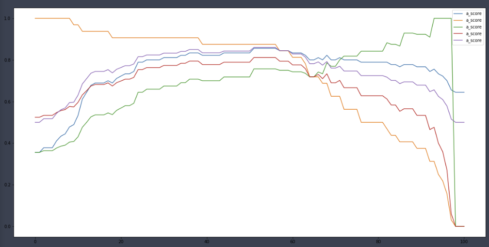

Wine quality

import pandas as pd
import numpy as np
import matplotlib.pyplot as plt
import seaborn as sns

df_white = pd.read_csv('./data/winequality-white (1).csv', sep=';')
df_red = pd.read_csv('./data/winequality-red (1).csv', sep=';')

df_red['redwhite'] = 0
df_white['redwhite'] = 1

df = pd.concat([df_red, df_white]) # 둘을 이어주지만 인덱스는 자신의 것을 그대로 사용하여 중복된 인덱스가 있을 것이다
df.reset_index(inplace=True) # 인덱스를 재조정한다
df.drop('index', axis=1, inplace=True)
df.isna().sum()

fixed acidity           0
volatile acidity        0
citric acid             0
residual sugar          0
chlorides               0
free sulfur dioxide     0
total sulfur dioxide    0
density                 0
pH                      0
sulphates               0
alcohol                 0
quality                 0
redwhite                0
dtype: int64

for i in df.columns:
    print('feature: ',i)
    if len(df.iloc[:,0].unique()) < 10:
        print(df[i].value_counts())
        plt.figure(figsize=(10,5))
        df[i].values_counts().plot(kind='bar')
    else:
        print(df[i].describe())
        plt.figure(figsize=(10,5))
        df[i].plot(kind='hist',bins=100)
    plt.show()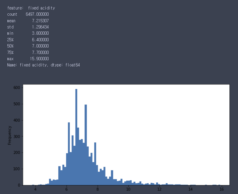

plt.figure(figsize=(10,10))
sns.heatmap(df.corr(), cmap='coolwarm', cbar=False, annot=True)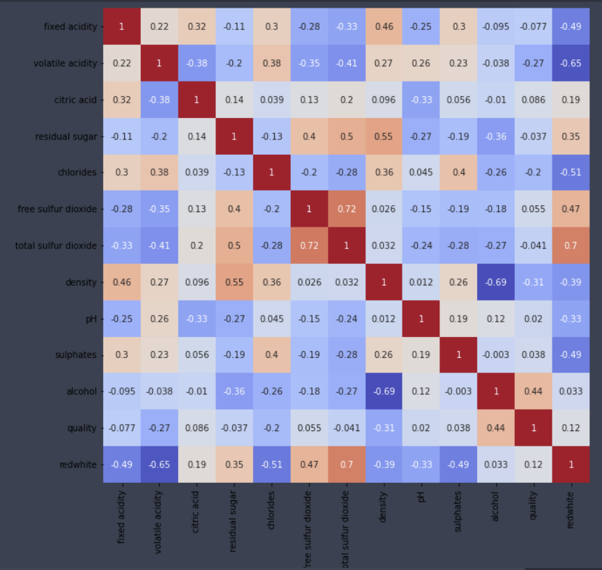

# 다중 분류 문제 -> 이진 분류 문제
df.quality.unique()

array([5, 6, 7, 4, 8, 3, 9], dtype=int64)

df['quality_new'] = 0
df.loc[df.quality > 6, 'quality_new'] = 1
df.quality_new.value_counts()

0    5220
1    1277
Name: quality_new, dtype: int64

df.drop('quality',axis=1, inplace=True)
for i in ['fixed acidity', 'volatile acidity', 'citric acid', 'residual sugar',
       'chlorides', 'free sulfur dioxide', 'total sulfur dioxide', 'density',
       'pH', 'sulphates', 'alcohol']:
    sns.violinplot(x='redwhite',y=i,hue='quality_new', data=df, inner='quartile',split=True)
    plt.show()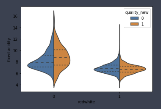

X = df.drop('quality_new', axis=1)
y = df.quality_new

X_train, X_test, y_train, y_test = train_test_split(X, y, test_size=0.1, random_state=42)

dt_clf = DecisionTreeClassifier()
rf_clf = RandomForestClassifier(n_jobs=2)
lr_clf = LogisticRegression(n_jobs=2)

rf_params = {'max_depth' : range(1, 11),
             'min_samples_leaf' : range(1, 11),
             'min_samples_split' : range(1, 11)}

dt_clf.fit(X_train, y_train)
rf_clf.fit(X_train, y_train)
lr_clf.fit(X_train, y_train)

dt_pred = dt_clf.predict(X_test)
rf_pred = rf_clf.predict(X_test)
lr_pred = lr_clf.predict(X_test)

def clf_eval(y_test, pred):
    confusion = pd.DataFrame(confusion_matrix(y_test, pred), 
                             columns=['예측 0','예측 1'], 
                             index=['실제 0', '실제 1'])
    accuracy = accuracy_score(y_test, pred)
    precision = precision_score(y_test, pred)
    recall = recall_score(y_test, pred)
    f_score = f1_score(y_test, pred)
    auc = roc_auc_score(y_test, pred)
    print('오차 행렬')
    print(confusion)
    print('-'*30)
    print('정확도: {0:.4f}, 정밀도: {1:.4f}, 재현율: {2:.4f}, F1스코어: {3:.4f}, AUC스코어: {4:.4f}'.format(accuracy, precision, recall, f_score, auc))

clf_eval(y_test, dt_pred)

오차 행렬
      예측 0  예측 1
실제 0   475    50
실제 1    51    74
------------------------------
정확도: 0.8446, 정밀도: 0.5968, 재현율: 0.5920, F1스코어: 0.5944, AUC스코어: 0.7484

clf_eval(y_test, rf_pred)

오차 행렬
      예측 0  예측 1
실제 0   508    17
실제 1    50    75
------------------------------
정확도: 0.8969, 정밀도: 0.8152, 재현율: 0.6000, F1스코어: 0.6912, AUC스코어: 0.7838

clf_eval(y_test, lr_pred)

오차 행렬
      예측 0  예측 1
실제 0   511    14
실제 1    97    28
------------------------------
정확도: 0.8292, 정밀도: 0.6667, 재현율: 0.2240, F1스코어: 0.3353, AUC스코어: 0.5987

dt_pred_prob = dt_clf.predict_proba(X_test)
rf_pred_prob = rf_clf.predict_proba(X_test)
lr_pred_prob = lr_clf.predict_proba(X_test)

a_score, r_score, p_score, f1score, auc = [], [], [], [], []
for i in range(1, 100):
    binarizer = Binarizer(threshold=i*0.01)
    dt_pred_new = binarizer.fit_transform(dt_pred_prob)[:,1]
    a_score.append(accuracy_score(y_test, dt_pred_new))
    r_score.append(recall_score(y_test, dt_pred_new))
    p_score.append(precision_score(y_test, dt_pred_new))
    f1score.append(f1_score(y_test, dt_pred_new))
    auc.append(roc_auc_score(y_test, dt_pred_new))
    
plt.figure(figsize=(20,10))
plt.plot(a_score, label='a_score')
plt.plot(r_score, label='r_score')
plt.plot(p_score, label='p_score')
plt.plot(f1score, label='f1_score')
plt.plot(auc, label='auc')
plt.legend()
plt.show()

a_score, r_score, p_score, f1score, auc = [], [], [], [], []
for i in range(1, 100):
    binarizer = Binarizer(threshold=i*0.01)
    rf_pred_new = binarizer.fit_transform(rf_pred_prob)[:,1]
    a_score.append(accuracy_score(y_test, rf_pred_new))
    r_score.append(recall_score(y_test, rf_pred_new))
    p_score.append(precision_score(y_test, rf_pred_new))
    f1score.append(f1_score(y_test, rf_pred_new))
    auc.append(roc_auc_score(y_test, rf_pred_new))
    
plt.figure(figsize=(20,10))
plt.plot(a_score, label='a_score')
plt.plot(r_score, label='r_score')
plt.plot(p_score, label='p_score')
plt.plot(f1score, label='f1_score')
plt.plot(auc, label='auc')
plt.legend()
plt.show()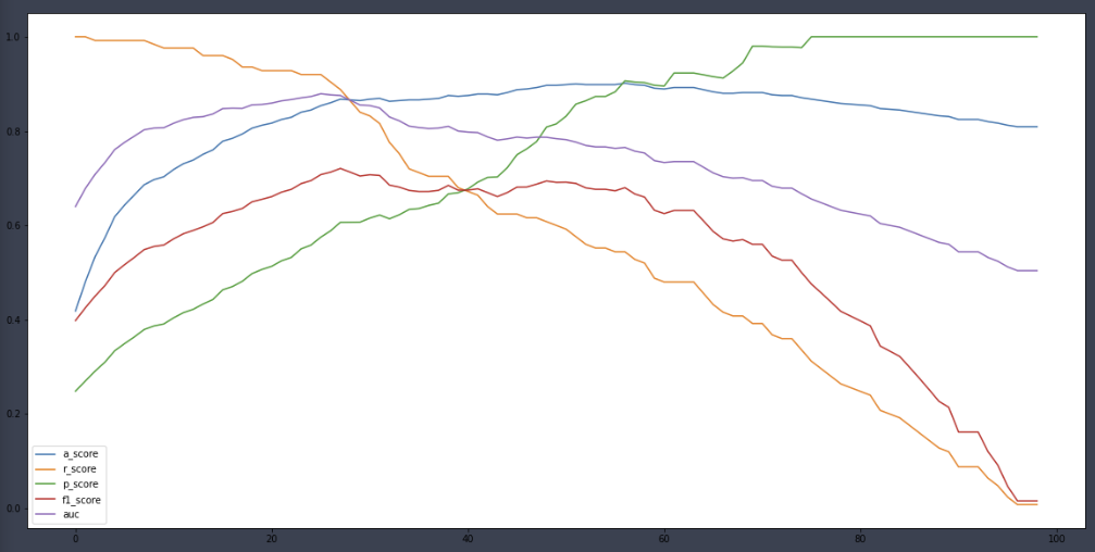

a_score, r_score, p_score, f1score, auc = [], [], [], [], []
for i in range(1, 100):
    binarizer = Binarizer(threshold=i*0.01)
    lr_pred_new = binarizer.fit_transform(lr_pred_prob)[:,1]
    a_score.append(accuracy_score(y_test, lr_pred_new))
    r_score.append(recall_score(y_test, lr_pred_new))
    p_score.append(precision_score(y_test, lr_pred_new))
    f1score.append(f1_score(y_test, lr_pred_new))
    auc.append(roc_auc_score(y_test, lr_pred_new))
    
plt.figure(figsize=(20,10))
plt.plot(a_score, label='a_score')
plt.plot(r_score, label='r_score')
plt.plot(p_score, label='p_score')
plt.plot(f1score, label='f1_score')
plt.plot(auc, label='auc')
plt.legend()
plt.show()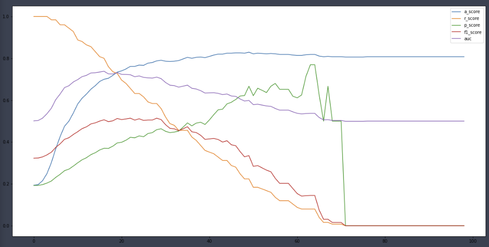

Decision Tree

구성

• 루트노드
• 규칙노드
• 리프노드

결정 트리는 규칙을 정할 때 균일도를 고려한다.

Gini Index

• 불순도 측정 계수
• 부모 노드의 Gini Index를 가장 많이 감소시키는 설명변수와 분리 값을 기준으로 자식노드를 형성
• 낮을수록 데이터의 균일도가 높음
• 낮은 속성을 기준으로 분할

Entrophy Index

• 데이터 집합의 혼잡도
• 서로 다른 값이 섞여 있으면 높고, 같은 값들이 많으면 낮음
• 부모 노드의 Entrophy Index를 가장 많이 감소시키는 설명변수와 분리값을 기준으로 자식 노드를 형성
• 낮을수록 균일도 높음

문제점

• 균일도가 0이 될 때까지 분기를 나누다보니 과적합 문제가 발생할 가능성이 높음
• 분기를 많이 할수록 학습데이터에 대해서는 완벽히 분류

제약

• 모델의 복잡도에 대한 제약을 학습 과정에 반영하는 것
• 학습데이터에 너무 과적합하여 새로 등장하는 데이터에 대한 예측 성능이 떨어지는 것을 방지
• 편향-분산 트레이드 오프

제약 파라미터

• 나무 구조 제한
  - 나무 깊이 제한: max_depth
  • 리프 노드 수 제한: max_leaf_nodes
• 불순도 기준
  - 분기를 발생시키는 최소 불순도 설정: min_impurity_split
  • 분기를 일으켰을 때, 최소한의 불순도 감소폭을 설정: min_impurity_decrease

장점

• 이해하기 쉬운 모델
• 피쳐 스케일링과 정규화 같은 전처리 영향이 크지 않음
• 명목형/연속형 모두 처리 가능

단점

• 과적합때문에 정확도가 떨어짐
• 이를 극복하기 위해 사전에 튜닝이 필요

from sklearn.tree import DecisionTreeClassifier
from sklearn.datasets import load_iris
from sklearn.model_selection import train_test_split
import warnings
warnings.filterwarnings('ignore')

# DecisionTree Classifier 생성
dt_clf = DecisionTreeClassifier(random_state=156)

# 붓꽃 데이터를 로딩하고, 학습과 테스트 데이터 셋으로 분리
iris_data = load_iris()
X_train , X_test , y_train , y_test = train_test_split(iris_data.data, iris_data.target,
                                                       test_size=0.2, random_state=11)

# DecisionTreeClassifer 학습. 
dt_clf.fit(X_train , y_train) 

from sklearn.tree import export_graphviz

# export_graphviz()의 호출 결과로 out_file로 지정된 tree.dot 파일을 생성함. 
export_graphviz(dt_clf, out_file="tree.dot", class_names=iris_data.target_names,
feature_names = iris_data.feature_names, impurity=True, filled=True)

import graphviz

# 위에서 생성된 tree.dot 파일을 Graphviz 읽어서 Jupyter Notebook상에서 시각화 
with open("tree.dot") as f:
  dot_graph = f.read()
graphviz.Source(dot_graph)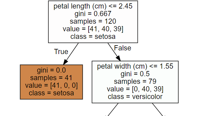

import seaborn as sns
import numpy as np
%matplotlib inline

# feature importance 추출
print("Feature importanes:\n{0}".format(np.round(dt_clf.feature_importances_, 3)))

# feature별 importance 매핑
# dictionary data 생성 {feature name: feature importance}
iris_fi = {}
for name, value in zip(iris_data.feature_names, dt_clf.feature_importances_):
  print('{0} : {1:.3f}'.format(name, value))
  iris_fi[name] = value

# items 데이터 생성 후 value 자리의 데이터로 내림차순 정렬
# key, value를 따로 저장
iris_fi_sorted = sorted(iris_fi.items(), key=lambda x: x[1], reverse=True)
iris_fi_sorted_feature = [feature for feature, importance in iris_fi_sorted]
iris_fi_sorted_importance = [importance for feature, importance in iris_fi_sorted]

# feature importance를 column 별로 시각화하기
# 가로막대 그래프는 반드시 내림차순으로 정렬할 것
sns.barplot(x=iris_fi_sorted_importance, y=iris_fi_sorted_feature)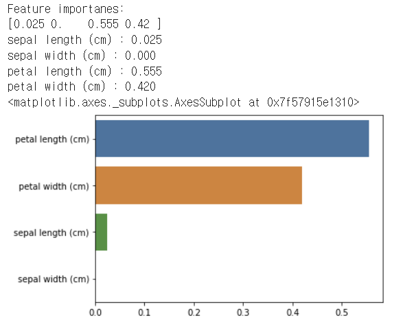 

과적합이 발생하면 feature importance는 신뢰도를 잃는다.

from sklearn.datasets import make_classification
import matplotlib.pyplot as plt
%matplotlib inline

plt.title("3 Class values with 2 Features Sample data creation")

# 2차원 시각화를 위해서 피처는 2개, 클래스는 3가지 유형의 분류 샘플 데이터 생성.
X_features, y_labels = make_classification(n_features=2, n_redundant=0, n_informative=2, n_classes=3, n_clusters_per_class=1, random_state=0)

# 그래프 형태로 2개의 피처로 2차원 좌표 시각화, 각 클래스 값은 다른 색깔로 표시됨.
plt.scatter(X_features[:, 0], X_features[:, 1], c=y_labels, s=25, edgecolor='k')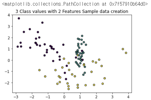

import numpy as np

# Classifier의 Decision Boundary를 시각화 하는 함수
def visualize_boundary(model, X, y):
  fig,ax = plt.subplots()
  
  # 학습 데이타 scatter plot으로 나타내기
  ax.scatter(X[:, 0], X[:, 1], c=y, s=25, cmap='rainbow', edgecolor='k',
             clim=(y.min(), y.max()), zorder=3)
  ax.axis('tight')
  ax.axis('off')
  xlim_start , xlim_end = ax.get_xlim()
  ylim_start , ylim_end = ax.get_ylim()
  
  # 호출 파라미터로 들어온 training 데이타로 model 학습 . 
  model.fit(X, y)
  # meshgrid 형태인 모든 좌표값으로 예측 수행. 
  xx, yy = np.meshgrid(np.linspace(xlim_start,xlim_end, num=200),np.linspace(ylim_start,ylim_end, num=200))
  Z = model.predict(np.c_[xx.ravel(), yy.ravel()]).reshape(xx.shape)
  
  # contourf() 를 이용하여 class boundary 를 visualization 수행. 
  n_classes = len(np.unique(y))
  contours = ax.contourf(xx, yy, Z, alpha=0.3,
                         levels=np.arange(n_classes + 1) - 0.5,
                         cmap='rainbow', clim=(y.min(), y.max()), zorder=1)

from sklearn.tree import DecisionTreeClassifier

# 특정한 트리 생성 제약 없는 결정 트리의 Decision Boundary 시각화.
dt_clf = DecisionTreeClassifier().fit(X_features, y_labels)
visualize_boundary(dt_clf, X_features, y_labels)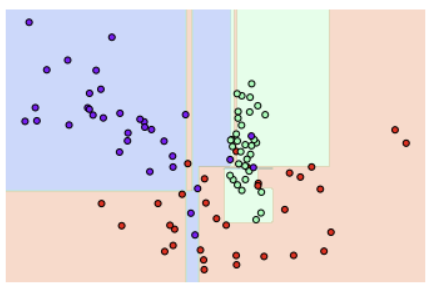

Ensemble

앙상블 모델

• 여러 머신러닝 기법을 합쳐서 하나로
• 단순/가중 평균
• Bagging (Bootstrap aggregating)
• Boosting
• Stacking == 메타학습

# 데이터 로드 및 패키지 임포트
# import Library
import pandas as pd
import seaborn as sns

from sklearn.ensemble import VotingClassifier, RandomForestClassifier
from sklearn.tree import DecisionTreeClassifier
from sklearn.linear_model import LogisticRegression
from sklearn.neighbors import KNeighborsClassifier
from sklearn.model_selection import train_test_split
from sklearn.metrics import accuracy_score
from sklearn.preprocessing import LabelEncoder

import warnings
warnings.filterwarnings('ignore')

df = sns.load_dataset('titanic')

df.drop(['embark_town', 'alive', 'class'], axis=1, inplace=True)
df.age.fillna(df.age.mean(), inplace=True)
df.embarked.fillna("N", inplace=True)
df.deck = df.deck.astype("object")
df.deck.fillna("N", inplace=True)

en_list = df.dtypes[(df.dtypes=='object') | (df.dtypes=='bool') | (df.dtypes=='category')].index
for i in en_list:
  encoder = LabelEncoder()
  encoder.fit(df[i])
  df[i] = encoder.transform(df[i])

# 입력데이터 X와 출력데이터 y를 분리
X = df.drop('survived', axis=1)
y = df.survived

# 개별 모델은 로지스틱 회귀와 KNN 임. 
lr_clf = LogisticRegression()
knn_clf = KNeighborsClassifier(n_neighbors=8)
dt_clf = DecisionTreeClassifier()
rf_clf = RandomForestClassifier()

# 개별 모델을 소프트 보팅 기반의 앙상블 모델로 구현한 분류기
vo_clf = VotingClassifier(estimators=[('LR', lr_clf),('KNN', knn_clf),
                                      ('DT', dt_clf)] , voting='soft')

X_train, X_test, y_train, y_test = train_test_split(X, y, test_size=0.2 , random_state= 156)

# VotingClassifier 학습/예측/평가. 
vo_clf.fit(X_train , y_train)
pred = vo_clf.predict(X_test)
print('Voting 분류기 정확도: {0:.4f}'.format(accuracy_score(y_test , pred)))

# 개별 모델의 학습/예측/평가.
classifiers = [lr_clf, knn_clf, dt_clf, rf_clf]
for classifier in classifiers:
    classifier.fit(X_train , y_train)
    pred = classifier.predict(X_test)
    class_name= classifier.__class__.__name__
    print('{0} 정확도: {1:.4f}'.format(class_name, accuracy_score(y_test , pred)))

Voting 분류기 정확도: 0.8436
LogisticRegression 정확도: 0.8212
KNeighborsClassifier 정확도: 0.7039
DecisionTreeClassifier 정확도: 0.8436
RandomForestClassifier 정확도: 0.8324

단순/가중 평균

• 여러 분류 모델이 예측한 결과를 가지고 다수결로 투표
• 생각보다 효과가 없다

Bagging

• Random Forest가 예시
• 데이터셋을 N개로 나눠서 각 모델에 전달하여 학습
• 모델이 Decision Tree면 Random Forest

Random Forest

• 앙상블 알고리즘
• 비교적 빠른 수행속도
• 다양한 영역에서 높은 예측 성능
• 결정 트리 기반
• 변수가 굉장히 많은 데이터 학습에 용이
• 과적합 문제
• Bagging이 편향을 줄이기는 어려움 (과소적합을 막기 어려움)

Hard Voting과 Soft Voting

• Hard Voting은 다수결
• Soft Voting은 각 모델이 내놓은 결과의 확률에 따라 결정

트리 기반 앙상블 알고리즘의 단점

• 하이퍼 파라미터가 너무 많음
• 튜닝을 위한 시간이 많이 소모
• 그럼에도 예측성능이 크게 향상되지 않는 경우가 많이 발생

Boosting

• 처음 예측을 하고, 틀린 것을 줄이는 방향으로 weight를 주고 다시 예측하는 것을 반복

Boosting이 Bagging에 밀렸던 이유

• 많은 계산량
• 튜닝해야 할 파라미터가 너무 많음
• Boosting은 분산 컴퓨팅이 어렵다

Gradient Boosting

• 장점
  - 과적합에도 강함
  • 뛰어난 예측 성능
• 단점
  - 수행시간이 오래 걸림
  

XGBoost (eXtreme Gradient Boost)

• 뛰어난 예측 성능
• GBM 대비 빠른 수행 시간
• 과적합 규제
• 가지치기
• 자체 내장된 교차 검증
• XGBoost는 10,000건 이하의 데이터에 사용하고, LGBM은 10,000건 이상의 데이터에 사용

언더 샘플링

• 많은 데이터를 적게 만드는 것
  - 0: 10,000건, 1: 100건 -> 0: 100건, 1: 100건
• 과도하게 정상 레이블로 학습/예측하는 부작용 개선
• 정상 레이블의 학습을 제대로 수행하기 어려운 단점
• 오버 샘플링은 반대로 적은 것을 많게 늘리는 것

Stacking

• m * n의 학습 데이터가 있을 때 각자 잘 만들어진 모델에 입력으로 넣는다
• 모델들의 학습할 때의 예측값으로 m * M(모델의 수)만큼의 행렬이 다시 생긴다
• m * M과 test를 이용해 second level model로 학습을 한번 더 수행