작성자 : 장아연

0. Recap

Deep Graph Encoder

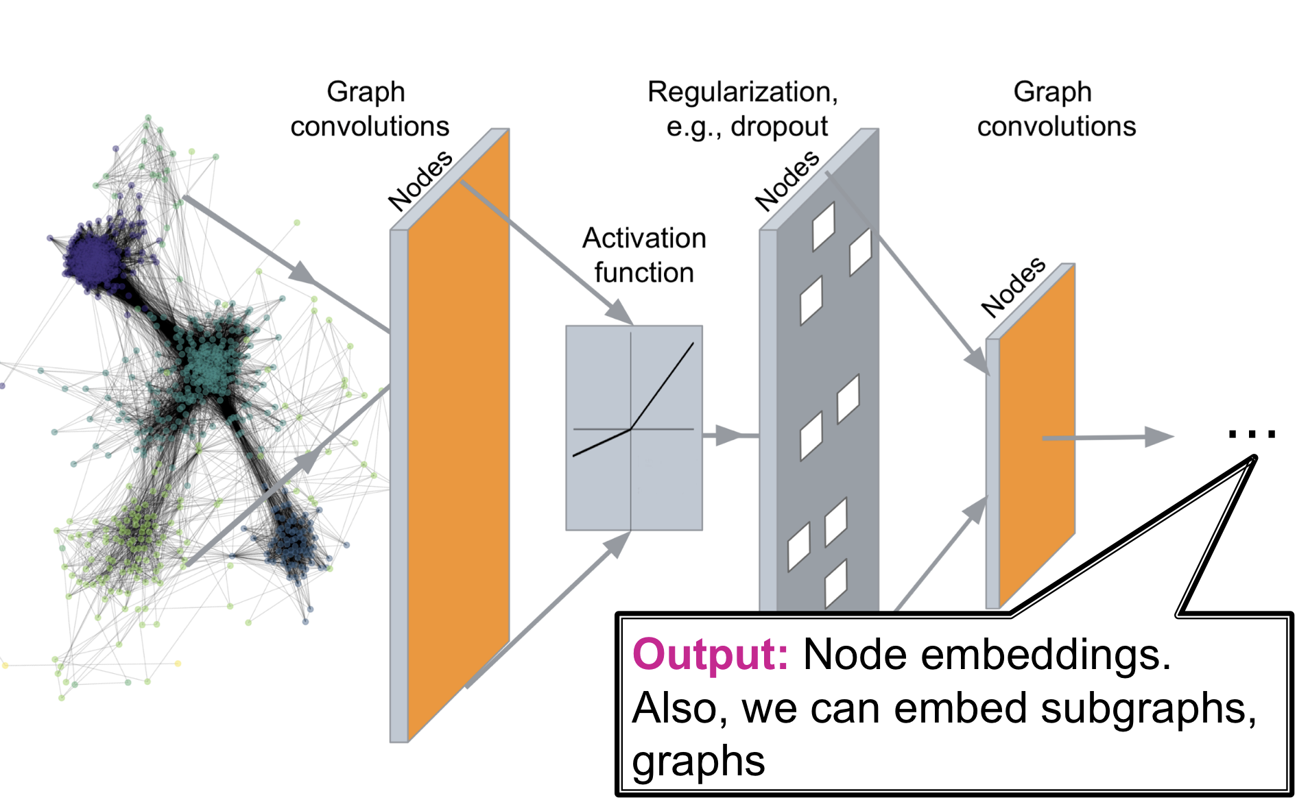
Deep Graph Encoders는 임의의 graph를 Deep Neural Network를 통과 시켜 embedding space로 사상 시키는 것

---

A General GNN Framework

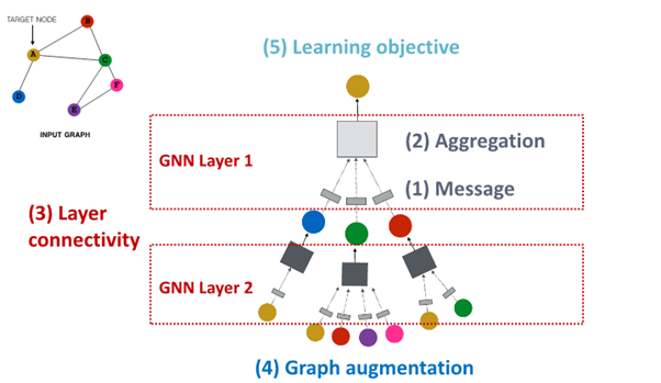
(4) Graph augmentation
: what kind of graph and feature augumentation can we create to shape the structure of this neural network
(5) Learning Objective
: learn objectives and how to make training work

---

1. Graph Augmentation for GNNs

Why Graph Augment

가정 : Raw input Graph 와 computational Graph는 동일

• Feature : lack features
• Graph Structure :
  sparse -> inefficient passing
  dense -> too costly passing
  large -> not computational graph into GPU
  즉, input graph는 embedding을 위한 computation graph의 적합한 상태가 아님.

Idea : Raw input Graph 와 computational Graph는 동일 X

Graph Augmentation Approaches

Graph Feature Augmentation

• lack features : feature augmentation을 통해 feature 생성

Standard Approach

필요성 : adj. matrix만 가지고 있는 경우 Input Graph에서 node feature가 없는 경우 흔히 발생

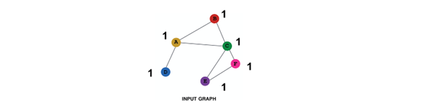
1. Constant Node Feature
Assign constant values to nodes
basically all the node have same future value of 1

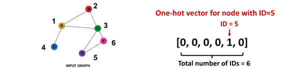
2. One-hot node feature
Assign unique IDs to nodes
IDs are converted to one-hot vectors
flag value 1 at ID of that single node

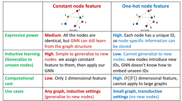
Constant Node Feature vs One-hot node feature

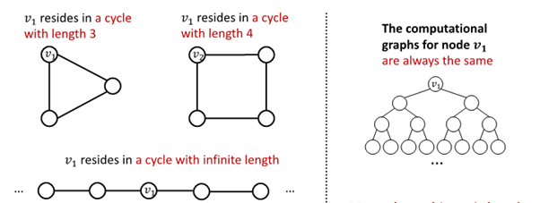
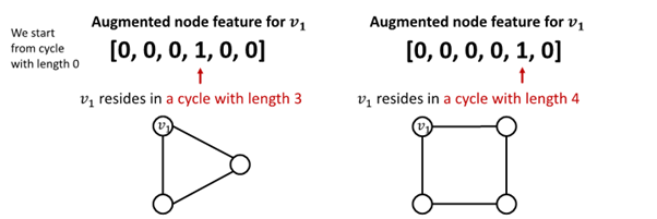
Cycle Count

필요성 : GNN 학습에 어려움을 겪는 특정 구조 존재

• GNN은 $\mathcal{v_1}$이 속한 cycle의 길이 학습 불가

• $\mathcal{v_1}$가 어떤 graph에 속해 있는지 구별 불가능

• 모든 node의 차수가 2임

• computational graph는 같은 binary tree임
  
  

• 그 외 Node Degree, Clustering coeffiecient, PageRank, Centrality 등 이용

Graph Structure Augmentation

• too sparse : virtual node / edges를 생성
• too dense : message passing 과정에서 neighbors sampling
• too large : embedding 계산을 위해 subgraph sampling

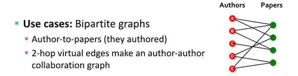
Add Virtual Edge

개념

• virtual edge를 이용해 2-hop 관계의 이웃 노드 연결
• adj.matrix 대신 $A+A^2$ 이용

예시

• Author(A)와 Author(B) 연결
  : Author(A) -> paper -> Author(B)
  

Add Virtual node

개념

• virtual node를 이용해 graph의 모든 node를 연결
• 모든 node와 node는 distance 2를 가짐
  : node(A) ->virtual node-> node(B)

예시

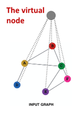
결과 : virtual node/edge 추가해 sparse한 graph에서 message passing 향상

Node Neighborhood Sampling

기존

• 모든 node는 message passing에 사용됨
  

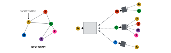
개념

• node neighborhood를 random sampling해 message passing 진행

예시 :
1. random하게 2개의 neighbor 선택해 sampling

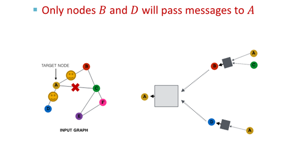
2. 다음 layer에서 다른 neighbor 선택해 resampling해 embedding 진행

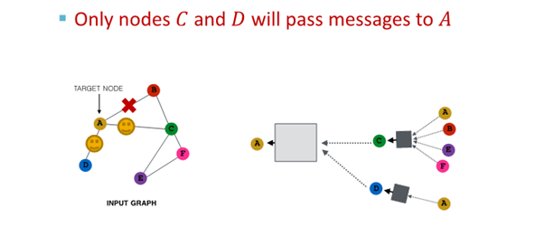
결과

• 모든 neighbor 사용한 경우와 유사한 embedding
• computational cost 경감
  (large graph scaling 해줌)
  

2. Prediction with GNNs

How to train GNN?

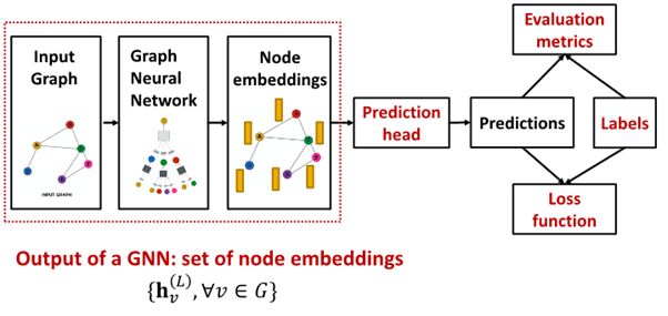
• $h_v^{(L)}$ : node L from graph neural network의 final layer
• Prediction head: final model's output
• Label : where label come from?
• Loss function : define loss function, what to optimize

Different Prediction Head

서로 다른 prediction head에 따라 서로 다른 task가 요구됨

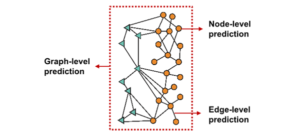
Node-level task

• node embedding 사용해 예측
• prediction head : { ${h_v^{(L)} \in \mathbb{R}^d,\forall_v \in G }$ }
  get $d$-dim node embedding from GNN computation
• $k$ way prediction의 경우
  classification : classify among $k$ categories
  regression : regress on $k$ target
• $\hat{y}_v$=$Head_{node}(h_v^{(L)})$=$W^{(H)}h_v^{(L)}$
  output head of given node=matrix time final embedding of node
• ${W^{(H)} \in \mathbb{R}^{k*d}}$ : $W^{(H)}$ map node embedding from ${h_v^{(L)} \in \mathbb{R}^d}$ (embedding space) to $\hat{y}_v \in \mathbb{R}^k$ (prediction)

Edge-level task

• node embedding pair 사용해 예측
  
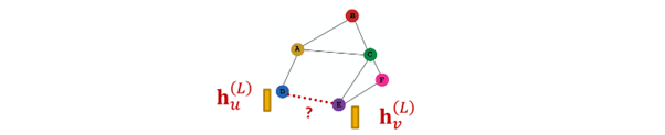
• $k$-way prediction의 경우 : $\hat{y}_{uv}$=$Head_{edge}(h_u^{(L)},h_v^{(L)})$

option for edge level prediction

1. Concatenation + Linear transformation

• $\hat{y}_{uv}$=$(h_u^{(L)})^Th_v^{(L)}$
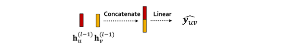
• $Linear$ : 2d-dimensional => $k$-dim embedding

2. Dot product

• $\hat{y}_{uv}$=$Linear(Concat(h_u^{(L)},h_v^{(L)}))$
• only applied to 1 way prediction (binary prediction)
• for $k$-way prediction : multi-head attention과 유사
  
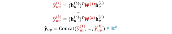
• trainable different matrix $W$ : $W^{(1)},$$W^{(2)}$ ... $W^{(k)}$ 이용
  => every class get to learn its own transformation
• prediction for every class인 $\hat{y}^{(1)}_{uv}$ ... $\hat{y}^{(k)}_{uv}$ 를 concat해 final prediction인 $\hat{y}_{uv}$ 구함

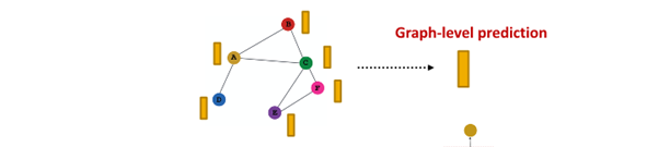
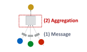
Graph-level task

• graph 속 모든 node embedding 이용해 예측
• $\hat{y}_G$=$Head_{graph}${ ${h_v^{(L)} \in \mathbb{R}^d,\forall_v \in G }$ }
  take individual node embedding for every node and aggregate them to find embedding in graph
  
• $Head_{graph}(*)$과 GNN에서 $AGG(*)$ 유사
  

option for Graph level prediction

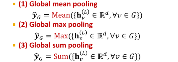
위 3개는 small graph에 적합함

large graph를 global pooling하여 information lose

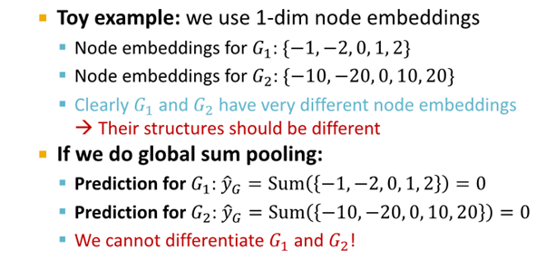
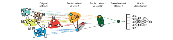
• solution : Hierarchical Global Pooling

Hierarchical Global Pooling

• 모든 node embedding을 위계 따라 aggregate

개념 예시

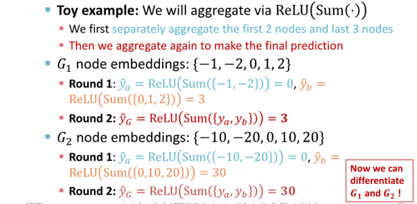
DiffPool idea : Hierarchically pool node embedding

3. Training Graph Neural Network

4. Setting - up GNN Prediction Tasks

Fixed split vs Random split

Fixed split

• Train : GNN parameters를 optimize에 사용
• Validation : model/hyperparameters를 develope
• Test : final performance를 report하는 데 사용
  -> test 결과에 대한 해당 실행 결과 보장X
  Random split
• randomly split training / validation / test dataset
  -> 서로 다른 random seed에 대해 performance를 average함

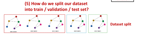
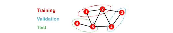
Why Splitting Graph is special

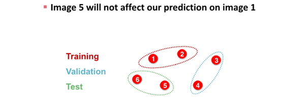
image data splite하는 경우

• image classification은 모든 data point가 image로 각각의 data가 서로 independent함
  

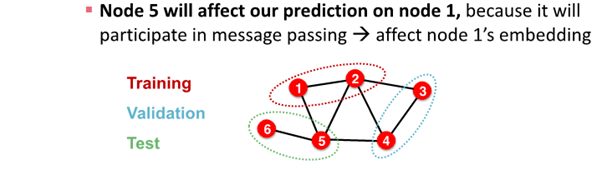
graph data splite하는 경우

• node classification은 모든 data point가 node로 각각의 data가 서로 dependent함
• node 1과 node 2는 node 5를 예측하는데 영향을 줌
  : node 1과 node2가 train data, node 5가 test data인 경우, information leakage 발생 가능
  

solution

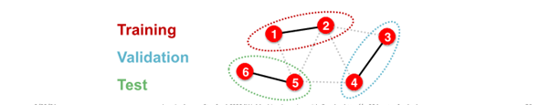
1. Transductive setting

• entire graph in all dataset
• only split label
• dataset consist of one graph
• node / edge prediction
• train : entire graph, use node 1 & 2 label
• validation : entire graph, use node 3 & 4 label
  

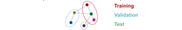
2. Inductive setting

• different graph in each dataset
• dataset consist of multiple graph
• generalize to unseen graph
• node / edge / graph task
• train : embedding 계산 graph over node 1 & 2, train use node 1 & 2 label
• validation : embedding 계산 graph over node 3 & 4, evaluate node 3 & 4 label
  

Example
1. Node Classification

• transductive node classification
  
• inductive node classification
  

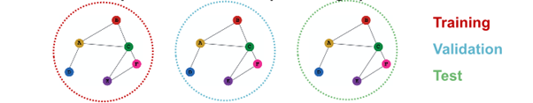
2. Graph Classification

• only in inductive setting
• test on unseen graph
  

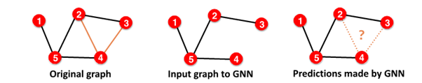
3. Link Classification

• predict missing edge
• unsupervised / self-supervised task
  -> create label & dataset split
  = we hide edge & let GNN predict whether edge exist
  

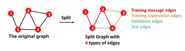
Setting up Link Prediction

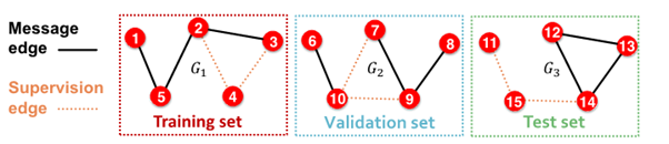
1-0. Assign edge as Message edges or Supervision edges

• Message edges : GNN message passing에 사용
• Supervision edges : objectives 계산에 사용

1-1.
message edges : remain in graph
supervision edges : supervise edge prediction made by model

2-0. split edges as train / validation / test
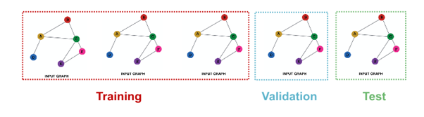
2-1. Inductive link prediction split의 경우

• contain independent graph in dataset
• 각 dataset에는 message edges와 supervision edges 가 포함됨
• supervision edges not fed in GNN
  
  2-2. Transductive link prediction split의 경우
• after train, supervision edges known to GNN
• use supervision edges at validation time
  
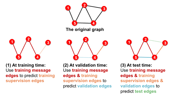
• in sum, 4 types of edges