Lec 02. Frequent Itemsets Mining

Yujin Kim·2022년 2월 28일

CS246 MMDS

CS246: Mining Massive Data Sets

목록 보기

1/1

Chapter 6 : Frequent Itemsets

the discovery of frequent itemsets =“association rules”를 발견하는 것!

<Course Outline>

1) “market-basket” model
2) First: Define
• Frequent itemsets
• Association rules: Confidence, Support, Interestingness
3) Then: Algorithms for finding frequent itemsets
• Finding frequent pairs
• A-Priori algorithm
• PCY algorithm

6.1. THE MARKET-BASKET MODEL

Baskets = “transactions”
items $\subset$ Basket

6.1.1 Definition of Frequent Itemsets

📎 “frequent”
⇒ $s$ , called the support threshold
I : set of items → support for I : I가 포함된 Basket의 수
if support for I > $s$ : I는 빈번하다(frequent)!

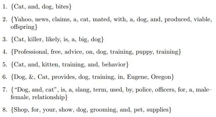
Example 6.1 :

Since the empty set is a subset of any set, the support for ∅ is 8.⇒ 하지만 일반적으로 공집합은 아무것도 말해주지 않기 때문에 신경쓰지 X
Example) “Dog”:(5)번을 제외 모든 basket에서 등장 ⇒ “Dog”의 support는 7
Suppose that we set our threshold at $s$ = 3 : Then there are five frequent singleton itemsets: {dog}, {cat}, {and}, {a}, and {training}
doubletons
- There are five frequent doubletons if s = 3; they are
  {dog, a} {dog, and} {dog, cat} {cat, a} {cat, and}
  - Each appears at least three times
frequent triple은 frequent doubletone의 조합으로만 가능
해당 예제에서는 하나의 frequent triple만 존재하므로,no frequent quadruples or larger sets.

6.1.2 Applications of Frequent Itemsets

: If someone buys diaper and milk, then he/she is likely to buy beer.

Related concepts: Let 1)items → words, and 2)baskets → documents (e.g., Web pages, blogs, tweets).

stopword를 제외하면, 공통 개념을 나타내는 두개의 단어 쌍이 자주 발견될 수 있음.

Plagiarism: Let 1)the items → documents and 2)the baskets → sentences. : An item/document is “in” a basket/sentence if the sentence is in the document.

we should remember that the relationship between items and baskets is an arbitrary many-many relationship : "in"은 "~의 일부"라는 전통적인 의미를 가질 필요가 없음.
여러 문장을 공유하는 두 개의 문서 → 표절의 좋은 지표!

Biomarkers: Let 1) the items be of two types – biomarkers such as genes or blood proteins, and diseases. 2) Each basket is the set of data about a patient: their genome and blood-chemistry analysis, as well as their medical history of disease.

질병 검사로 활용 가능

6.1.3 Association Rules

: extracting frequent sets of items from data = association rules라고 부르는 if-then 규칙의 모음으로 표시

* association rules

form : $I → j$ , where $I$ : set of items, $j$ : an item
$\{i_1, i_2,…,i_k\} → j$ means: “if a basket contains all of $i_1,…,i_k$ then it is likely to contain $j$ ”
In practice there are many rules, want to find significant/interesting ones!
1) Defining the confidence of the rule $I → j$

📌 conf( $I → j$ ) $\overset{\underset{\mathrm{def}}{}}{=}$ $\frac{\mathsf{support\ } (I ∪ \{j\})} {\mathsf{support\ } (I)}$

: $j$ 가 포함되는 모든 basket $I$ 의 비율

= support(I) is given → how often does $j$ appear next to it?

$= P(j|I) = \frac{P(I,j)}{P(I)}$

Example) Fig 6.1에서
The confidence of the rule {cat, dog} → and = 3/5.
- {cat, dog}이 언급된 basket의 support = 5
- {cat, dog}이 and 와 함께 언급된 basket = 즉, {cat, dog, and}의 support = 3
$I$ 의 support가 매우 크다면, confidence 하나만으로도 매우 useful 할 수 있음.
However, I가 $j$ 에 (어떻게든) 영향을 미치는 실제 관계에서는 Association Rule이 더 중요함.
2) Thus, define the interest of an association rule $I → j$ : (rule $I → j$ 의 confidence)와 ( $j$ 를 포함하는 basket의 비율)의 차이

📌 $Interest(I → j) =| conf(I → j) - Pr[j]|$
- if I가 j에 영향을 미치지 않는다면,
  ${I\mathsf{와}\ j\mathsf{를}\ \mathsf{포함하는\ basket} \over I\mathsf{를\ 포함하는\ basket}} = {j\mathsf{를\ 포함하는\ basket} \over \mathsf{모든\ basket}}$
  → rule의 interest = 0
  - Example) I가 있으면 항상 J가 따라오는 경우 → not very interesting!
- rule이 high(+) interest = basket의 I가 → j가 존재하는 것을 유발함
  - the rule $\{diapers\} → beer$ has high interest.
- rule이 highly negative(-) interest = basket의 I가 → j가 존재하는 것을 억제함을 알 수 있음.
  - the rule $\{pepsi\} → coke$ can be expected to have negative interest.
- interest가 매우 낮거나 매우 높은 경우 → 둘다 interesting!

6.1.4 Finding Association Rules with High Confidence

basket의 합리적인 정도(reasonable fraction)에 적용되는 Association Rules $I → j$ 를 찾기 위해서는,

1) I의 support가 상당히(reasonably) 높아야 한다.

오프라인 매장에서의 마케팅과 같이 실제로 “reasonably high”한 비율은 종종 바구니의 약 1%

2) rule의 confidence 상당히 높아야 한다.

usually above 0.5 = 50%, 그렇지 않으면 규칙이 실제 효과가 거의 X
결과적으로 집합 $I ∪ \{j\}$ 도 상당히 높은 support를 가져야 함.

💡 Problem: Find all association rules with support ≥s and confidence ≥c

→ This means: support( $I ∪ \{j\}$ ) $\ge s$ ⇒ Conf $\ge c$

why?

Note: Support of an association rule is the support of the set of items in the rule (left and right side)
Hard part: Finding the frequent itemsets!

Suppose) 1. s와 c : given to us by user or by the data analyst.

threshold of support( $s$ )를 달성하는 모든 itemsets를 찾았고, 각 itemset에 대한 support를 계산했다고 가정 → 빠르게 conf 계산 가능

→ 높은 support && 높은 confidence를 가진 Association Rules를 찾을 수 있음

That is) if $J$ 가 frequent( $\ge s$ )한 $n$ 개의 items을 가지고 있다면,
→ only n possible association rules involving this set of items
= $J$ 에 존재하는 모든 $j$ 에 대하여 $J − \{j\} → j$ (총 n개 존재)

→ $J$ 가 frequent( $\ge s$ ) 이면, $J − \{j\}$ 도 frequent( $\ge s$ )

Why? If $\{i_1, i_2,…, i_k\} → j$ has high support and confidence, then both $\{i_1, i_2,…, i_k\}$ and $\{i_1, i_2,…,i_k, j\}$ will be “frequent”

⇒ $J$ 와 $J − \{j\}$ 의 support 비율
= 규칙 $J − \{j\} → j$ 의 신뢰도 = $\frac{\mathsf{the\ support\ for\ } J-\{j\} ∪ \{j\}} {\mathsf{the\ support\ for\ } J-\{j\}}$ = $\frac{\mathsf{the\ support\ for\ } J} {\mathsf{the\ support\ for\ } J-\{j\}}$

Assumed that) there are not too many frequent itemsets and thus
not too many candidates for high-support, high-confidence association rules. → 너무 많은 frequent itemsets을 얻지 않도록 support threshold( $s$ )를 조정하는 것이 일반적!

* How to make Algorithm ?

Step 1) Find all frequent itemsets $I$
(we will explain this next)

Step 2) Rule generation

For every subset

A

I

, generate a rule

A → I \setminus A

Since I is frequent, A is also frequent
- Variant 1: Single pass to compute the rule confidence
confidence(A,B→C,D) = support(A,B,C,D) / support(A,B)
- Variant 2:
- Observation: If A,B,C→D is below confidence, so is A,B→C,D

        why? support({A,B}) > support({A,B,C})
        conf(A,B,C→D) = support(A,B,C,D) / support(A,B,C)
        conf(A,B→C,D) = support(A,B,C,D) / support(A,B)
        
        $\therefore$  in every case, conf(A,B,C→D) < conf(A,B→C,D)
        
    - Can generate “bigger” rules from smaller ones!
    Output the rules above the confidence threshold

→ Finding Frequent Itemsets

Itemsets Computation Model
- The true cost of mining diskresident data is usually the number
  of disk I/Os : disk에 저장된 파일을 처음~끝까지 읽어내리는 시간!
- Bottleneck : main-memory
- Question : How do we know if something cannot be frequent if we haven’t counted it yet?

1) Naive Algorithm : data file을 한번 스캔하여 각 pair가 몇번 등장하는지 count한다. → impossible

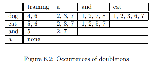
2) Counting Pairs in Memory

Approach 1) Triangular Matrix : Dense

장점; 4 bytes per every pair
단점; preallocating every element

Approach 2) Triples : Sparse

장점; preallocating nothing
단점; 12 bytes per occuring pair

→ “how many different pairs actually occured in the data”에 따라 사용할 방법 결정.

all possible pairs almost all occur : App1
lots of items, but only few pairs tent to occur : App2

& Approach 2 beats Approach 1 if less than 1/3 of possible pairs actually occur. (가능한 쌍의 1/3 미만이 발생할 경우 App2가 더 효율적)

💥 Problem : if we have too many items so the pairs do not fit into memory. Can we do better? → A-Priori Algorithm !

6.2 Market Baskets and the A-Priori Algorithm

Key idea : Monotonicity of Frequent

⇒ if set of items $I$ 가 최소 $s$ 번 나타난다면, $I$ 의 subset $J$ 도 최소 $s$ 번 나타남. J가 less frequent 할 수 없음.

대우 ⇒ if item $i$ 가 $s$ 개의 basket에서 나타나지 않는다면(support threshold를 넘지 못한다면), $i$ 를 포함하는 모든 집합은 $s$ 를 넘을 수 없음.

method : frequent singletones to frequent pairs!

Pass 1)Read baskets and count in main memory the # of occurrences of each individual item

→ Items that appear $≥s$ times are the frequent items

Pass 2) Read baskets again and keep track of the count of only those pairs where both elements are frequent (from Pass 1)

→ Requires memory proportional to square of frequent items only (not all items)

→ K-tuple로 일반화 가능

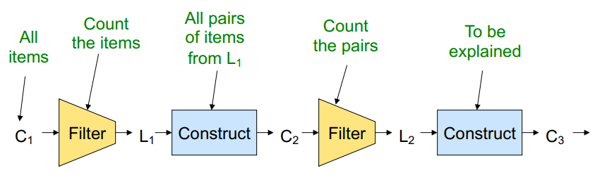
: single → pairs → triples → ... k-tuples

Example)

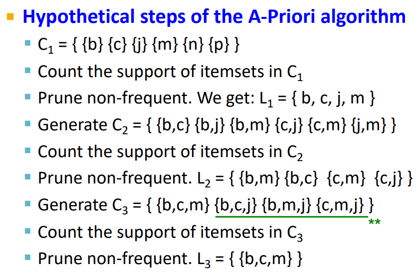
C3의 {b,c,j} {b,m,j} {c,m,j} 는 non-frequent 할 수밖에 없음

why? {b,c,j}에서 {b,c}와 {c,j}는 frequent하지만, {b,j}는 frequent하지 않음. (by L2)

⇒ {b,c,j}는 frequent할 수 없으므로, generate하지 않아도 됨.

6.3 Handling Larger Datasets in Main Memory

→ to cut down on the size of candidate set $C_2$

6.3.1 PCY(Park, Chen, and Yu) Algorithm

= Also known as “DHP(Direct Hashing and Pruning)”

Pass 1

FOR (each basket) :
		FOR (each item in the basket) :
				add 1 to item’s count;
		<!-- new in PCY , Hashing Process -->
		FOR (each pair of items) :
				hash the pair to a bucket;
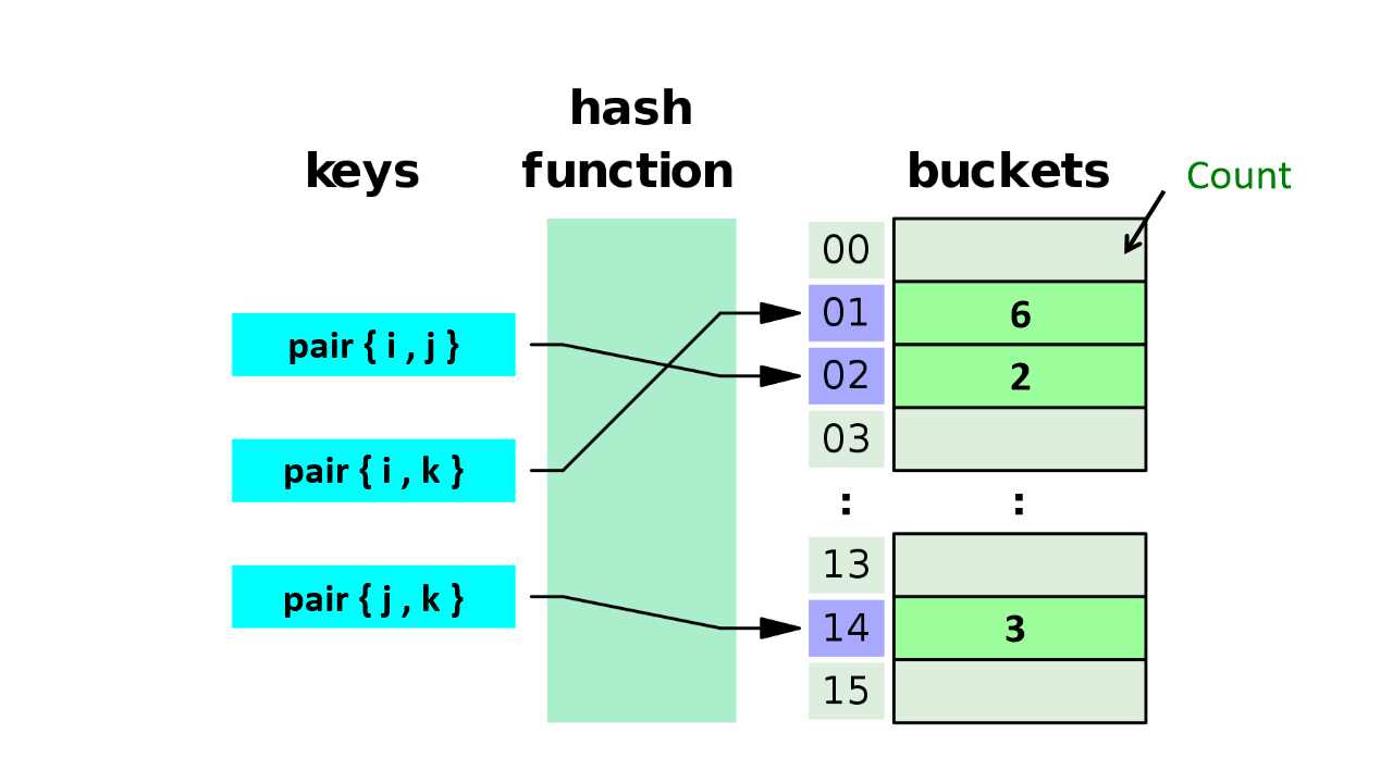
				add 1 to the count for that bucket;

PCY - Hash Table

keys : Pairs
buckets : integers(Count)

Between Passes

Observation:

1) If a bucket contains a frequent pair, then the bucket is surely frequent

However, even without any frequent pair, a bucket can still be frequent ☹️
§ So, we cannot use the hash to eliminate any member (pair) of a “frequent” bucket

2) But, for a bucket with total count less than $s$ , none of its pairs can be frequent 🙂

Pairs that hash to this bucket can be eliminated as candidates (even if the pair consists of 2 frequent items)
Pass 2: Only count pairs that hash to frequent buckets

cf> hash table을 만들 때, (메모리가 충분하다면) 가능한 fewer collision을 만드는 것이 좋음!

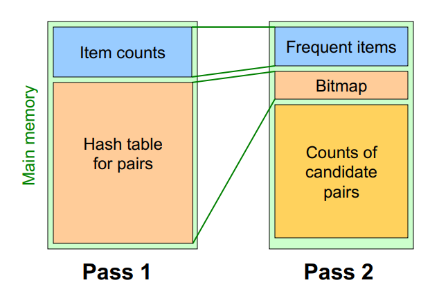
implementation : Replace the buckets by a bit-vector!

→ 1 means the bucket count exceeded the support $s$ (call it a frequent bucket); 0 means it did not

→ count를 위한 4byte Integer 가 bit-vector로 대체되면서 1/32 메모리만 사용 가능!

pass1에서 pass2로 넘어가면서 hash table이 frequent bucket인지 여부( $\ge s$ ) 를 Bitmap으로 기록.
Pass 2

Count all pairs {i, j} that meet the conditions for being a candidate pair:

Both $i$ and $j$ are frequent items
The pair {i, j} hashes to a bucket whose bit in the bit vector is 1 (i.e., a frequent bucket)

⇒ 두가지 조건이 모두 만족되면 Tracking :
Both conditions are necessary for the pair to have a chance of being frequent.

* Example

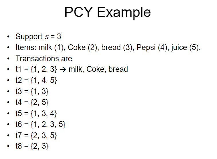
Pass 1 :

Item’s Count : 각 item이 몇번 등장하는지 count한다.
- Hash Table 아님
* Item Count 결과

Item Count
1 5
2 5
3 6
4 2
5 4
- item4는 $s$ 를 넘지 못함.
Make Hash Table for bucket counts
1. step 1) 모든 basket의 가능한 Pair를 생성
2. step 2) 각 Pair를 Hash Table에 해싱
  
  → 여기서는 Hashing Rule을 다음과 같이 정의
  : Hashing a pair {i, j} to a bucket k, where k = hash(i, j) = (i + j) / 5
  
  예를 들어, {1,2}를 hashing한다면 (1+2)/5 = 3 이니까 3번 bucket에 hashing됨.
```
(1, 4) and (2, 3) ->  k = 0
(1, 5) and (2, 4) ->  k = 1
(2, 5) and (3, 4) ->  k = 2
(1, 2) and (3, 5) ->  k = 3
(1, 3) and (4, 5) ->  k = 4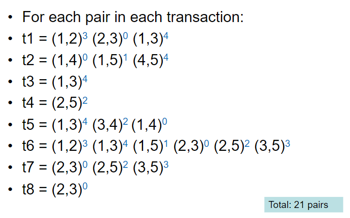
```
* Hash Table 결과

Bucket Count
0 6
1 2
2 4
3 4
4 5
- 1번 버킷으로 hashing되는 pair는 t2의 (1,5)와 t6의 (1,5)만 존재 → Count : 2
- 1번 버킷에 속하는 pair는 $s$ 를 넘지 못함.
  → 1번 버킷에 속하는 (1,5)와 (2.4)는 not frequent!

Item	Count
1	5
2	5
3	6
4	2
5	4

Bucket	Count
0	6
1	2
2	4
3	4
4	5

Pass 2 :

Frequent items : {1,2,3,5} (By Pass 1 - item’s count)

→ 이에 따라서, 가능한 candidate pair는 (1,2) (1,3) (1,5) (2,3) (2,5) (3,5)

⭐ (1,5)는 폐기 : because bucket 1 is not frequent! (By Pass 1 - hash Table)

→ Surviving Pairs = (1,2) (1,3) (2,3) (2,5) (3,5)

→ Counts of the Surviving Pairs

Pair	Count
(1,2)	2
(1,3)	4
(2,3)	4
(2,5)	3
(3,5)	2

(1,2) (3,5)는 $s$ 를 넘지 못함

⇒ Result : Frequent itemsets are {1} {2} {3} {5} {1,3} {2,3} {2,5}

The MMDS book covers several other extensions beyond the PCY idea: “Multistage” and “Multihash”

Recommended video (starting about 10:10): https://www.youtube.com/watch?v=AGAkNiQnbjY

6.4 Limited-Pass Algorithms

: Can we use fewer passes? ( in $\le k$ passes)

* Frequent Itemsets in $\le 2$ Passes

Use 2 or fewer passes for all sizes,but may miss some frequent itemsets

Random sampling
SON (Savasere, Omiecinski, and Navathe) Algorithm
Toivonen Algorithm

6.4.1 The Simple, Randomized Algorithm

: 1) Take a random sample of the market baskets
→ 2) Run a-priori or one of its improvements in main memory

장점 : Disk I/O 시간 필요 X
Sample size에 맞게 support threshold( $s$ )를 감소시켜야 함.
- Example) if your sample is 1/100 of the baskets, use $s/100$ as your support threshold instead of $s$ .
- Smaller threshold, e.g., $s/125$ , helps catch more truly frequent itemsets (But requires more space)
To avoid false positives: 추가로, candidate pairs가 전체 데이터에 대해서 frequent한지 확인하기 위해서 second pass에서 추가로 sampling한 데이터를 가지고 검증!

6.4.4 The SON Algorithm and MapReduce

: Repeatedly read small subsets of the baskets into main memory and run an in-memory algorithm to find all frequent itemsets

Note: Sampling 방법과 비슷하지만, sampling하는 것 아님(6.1.1과 다르게), but 모든 file data를 in memory-sized chunks로 쪼갬.

Path 1) An itemset becomes a candidate if it is found to be frequent in any one or more subsets of the baskets. (: make Candidate itemsets)

pass 2) count all the candidate itemsets and determine which are frequent in the entire set.(: Verify)

→ SON 알고리즘은 병렬 컴퓨팅 환경에 적합. 각 pass를 MapReduce 작업으로 표현하여 두 단계의 MapReduce-MapReduce 시퀀스로 실행시킬 수 있음.

6.4.5 Toivonen’s Algorithm

Pass 1)

Start with a random sample
- but lower the threshold( $s$ ) slightly for the sample
Find frequent itemsets in the sample
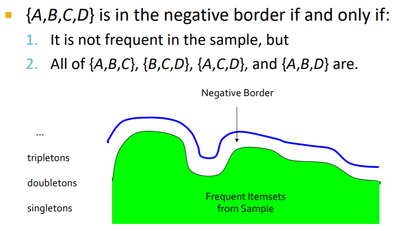
construct the negative border
- Negative border : An itemset is in the negative
  border if it is not frequent in the sample, but all its immediate subsets are frequent.
- Immediate subset = “delete exactly one element”

Pass 2) new sampling → Count all candidate frequent itemsets from the first pass, and also count sets in their negative border.

If no itemset from the negative border turns out to be frequent, then we found all the frequent itemsets.
What if we find that something in the negative border is frequent?
→ We must start over again with another sample!

※ 대체로, Pass 1에서는 frequent할 수 있는 candidate pairs를 만들고 → Pass 2는 candidate들을 전체 dataset에 대해서 verify 하는 알고리즘!

Yujin Kim