<Course Outline>

1. Why Graphs
2. Applications of Graph ML
3. Choice of Graph Representation

1.1 - Why Graphs

: Graphs are a general language for describing and analyzing entities with relations/interactions.

Types of Networks and Graphs

1. Networks ( = Natural Graphs, 자연적으로 그래프 구조로 생긴 것)
   • Social networks
   • Communications and transactions
   • Biomedicine (genes/proteins)
   • Brain connections
2. Graphs (as a representation of relational structure, 관계를 표현하기 위해 그래프로 모델링 한 것)
   • Information/knowledge
   • Software
   • Similarity networks: Connect similar data points
   • Relational structures: Molecules, Scene graphs, 3D shapes, Particle-based physics simulations

💡 Main question : How do we take advantage of relational structure for better prediction?
복잡한 + 많은 관계를 relational graph로 모델링함으로써 더 좋은 성능을 기대할 수 있음!

⇒ But, 현대의 딥러닝 기법은 단순한 sequences & grid 구조의 데이터 타입을 위해 디자인 됨.

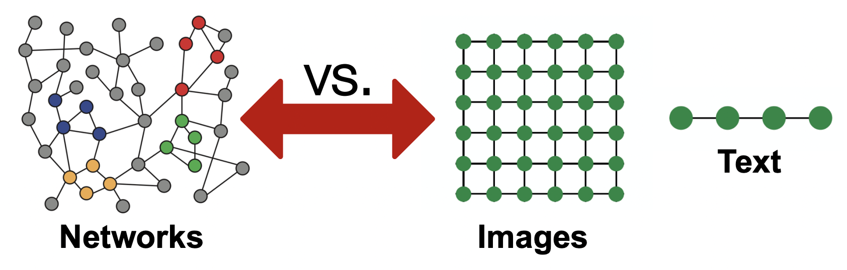
대표적으로 sequence & grid한 데이터 구조인 Images / Texts 에 비해 네트워크는 더 복잡한 구조를 가지고 있음

• 크기가 다양하고, 복잡한 모양을 가짐
• 위, 아래, 왼쪽, 오른쪽과 같은 공간상의 위치(spartial locality)가 없음
• 정해진 순서나 (출발점 같은) 기준점이 없음
• dynamic하며 multimodal features를 동시에 포함하기도 함

This Course ...

💡 question : 어떻게 하면 Graph와 같은 complex한 data에 딥러닝을 적용할 수 있을까?

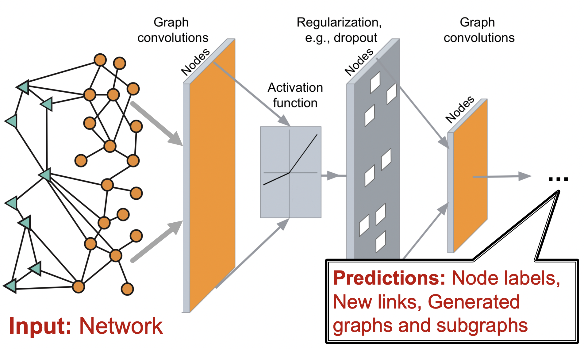
• input : Network
• output : Predictions

위 과정을 End-to-End로 할 수 있는 neural network architecture를 디자인

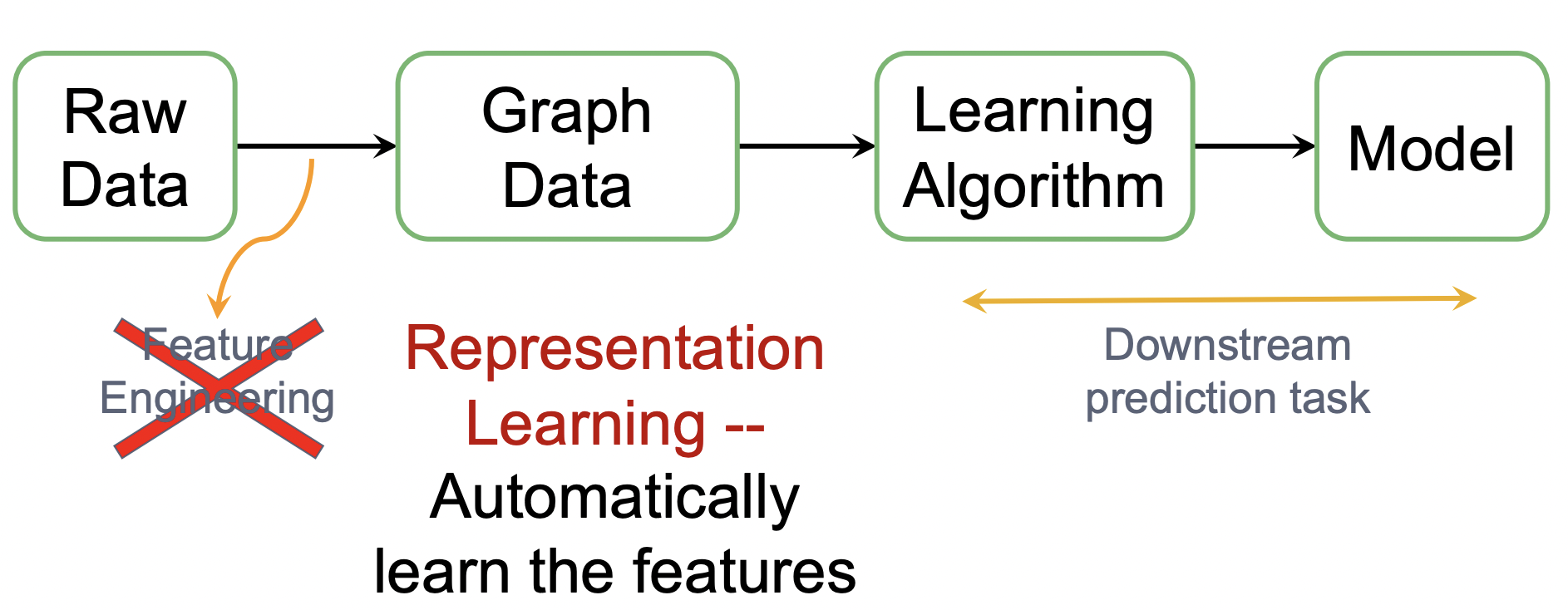
엔지니어가 적절한 feature를 디자인 하는데 많은 노력이 필요했던 전통적인 Feature Engineering (사용 X) → 그래프를 통해 downstream prediction task에 필요한 피처를 자동으로 학습하는 Representation Learing (O)

Representation Learning이란?

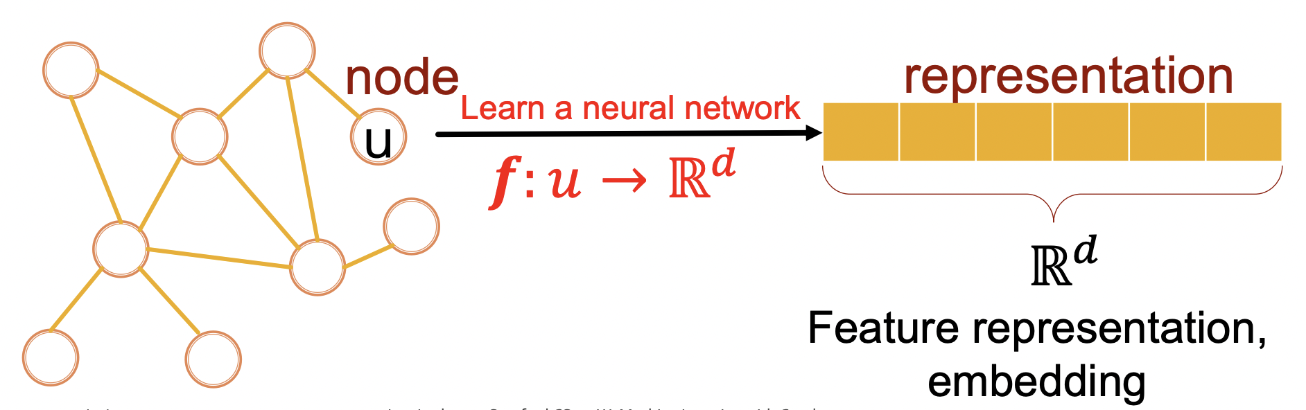
• 그래프의 node를 d-demensional vector로 임베딩
• 유사한 노드가 Embedding Space에 가까이 위치하도록 매핑

1.2 - Applications of Graph ML

Classic Graph ML Tasks

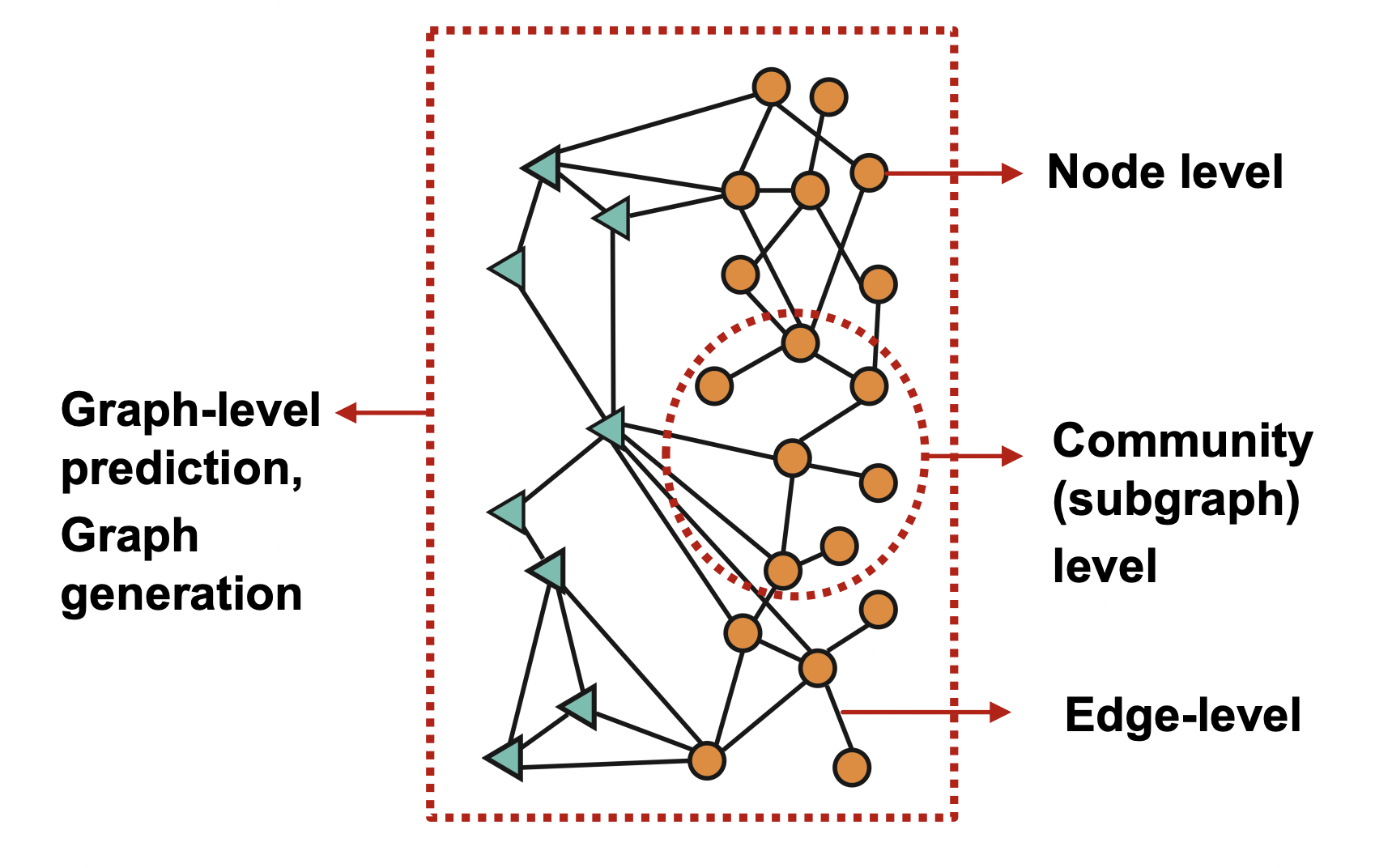
1. Node-level ML Tasks (Node classification): Predict a property of a node
   • Example:
     1. Categorize online users / items
     2. Protein Folding (e.g. AlphaFold) : 공간 상에서 노드의 위치를 예측
2. Edge-level ML Tasks (Link prediction): Predict whether there are missing links between two nodes
   • Example:
     1. Knowledge graph completion
     2. Recommender systems (e.g. PinSage): user-item interaction 예측
     3. Given a pair of drugs → predict adverse side effects
3. Subgraph-level ML Tasks:
   1. Traffic Prediction
   2. Clustering: Detect if nodes form a community
      • Example: Social circle detection
4. Graph-level ML Tasks:
   1. Graph generation: Drug discovery
      • Example:
        1. Antibiotic Discovery
        2. Molecule Generation / Optimization
   2. Graph evolution: Physical simulation
   3. Graph classification: Categorize different graphs
      • Example: Molecule property prediction

: 데이터 및 가능한 경우의 수가 많을 때 verify할 가치가 있는 Testset을 빠르게 찾는 Simulator의 역할

1.3 - Choice of Graph Representation

Components of a Network

• Objects: nodes, vertices : denoted as $N$
• Interactions: links, edges : denoted as $E$
• System: network, graph : denoted as $G(N,E)$

How to build a graph:

• What are nodes?
• What are edges?

⇒ Choice of the proper network representation of a given domain/problem determines our ability to use networks successfully: The way you assign links will determine the nature of the question you can study

Directed vs. Undirected Graphs

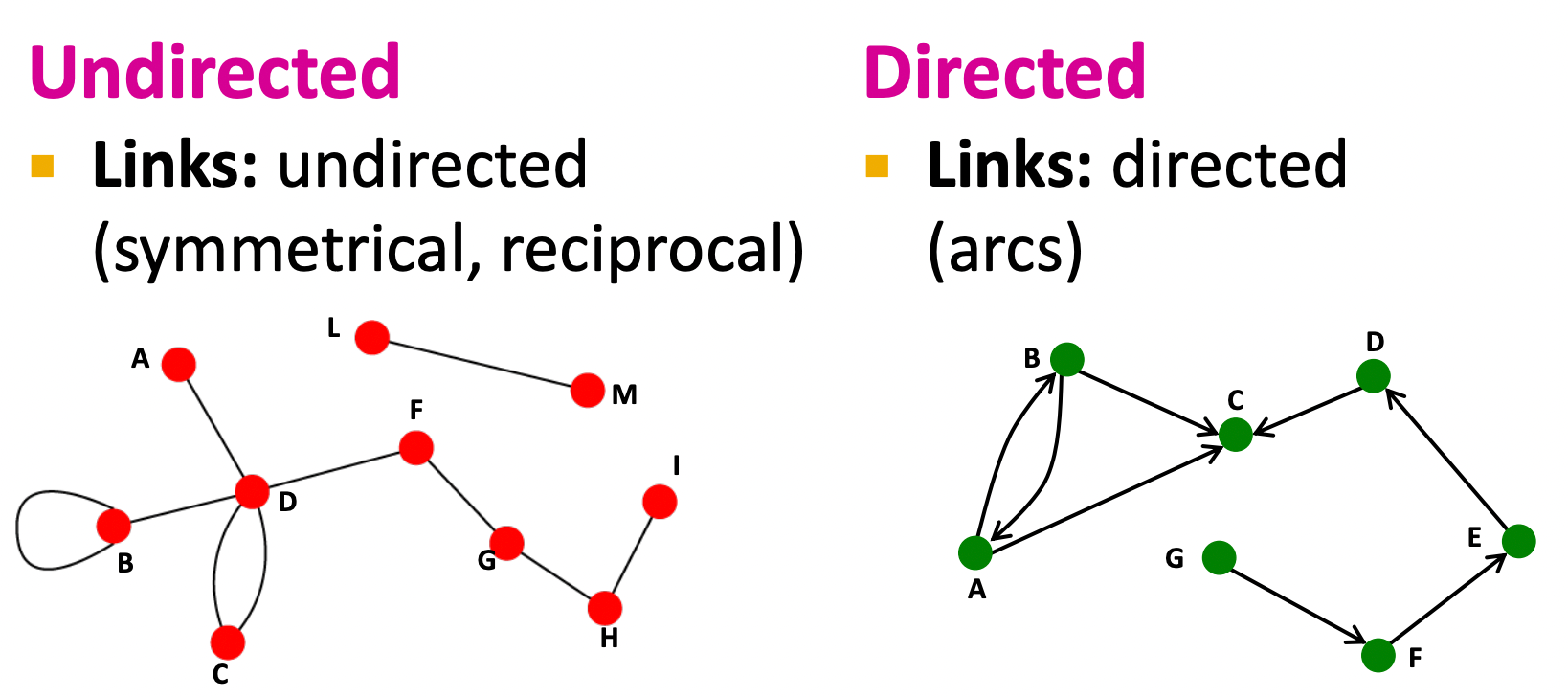
1) Directed

• Node degree, $k_i$ : node $i$ 와 인접한(연결된) 엣지의 개수
• Avg. degree : $\bar{k} = \left\langle k \right\rangle = \frac{1}{N} \sum_{i=1}^N k_i = \frac{2E}{N}$

2) Undirected

• source → destination 이 존재
• in-degree, $k_c^{in}$
  out-degree, $k_c^{out}$
• total degree, $k_c$ = $k_c^{in} + k_c^{out}$
• Avg. degree = $\frac{E}{N}$
  • $\bar{k_c^{in}} = \bar{k_c^{out}}$
• Source: Node with $k^{in}$ = 0
  Sink: Node with $k^{out}$ = 0

Bipartite Graph (이분 그래프)

: 두가지 diffirent types의 노드 종류를 가지며, 오직 다른 종류의 노드와 상호작용(같은 종류의 노드끼리는 연결되지 않음)하는 그래프를 말함.

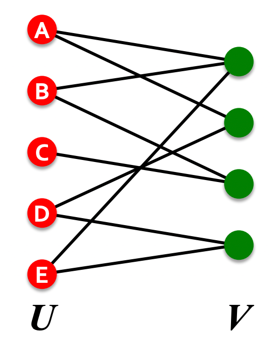
→ 이를 Folded Network 개념으로 나타낼 수 도 있음.

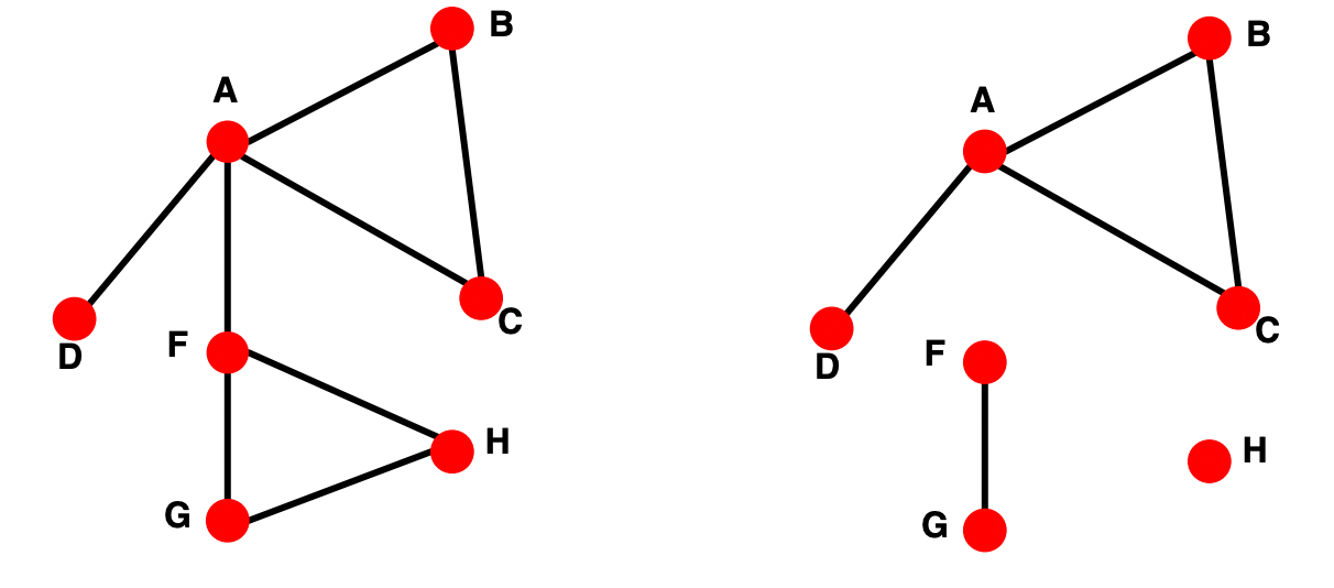
Folded(=Projected) Bipartite Graphs

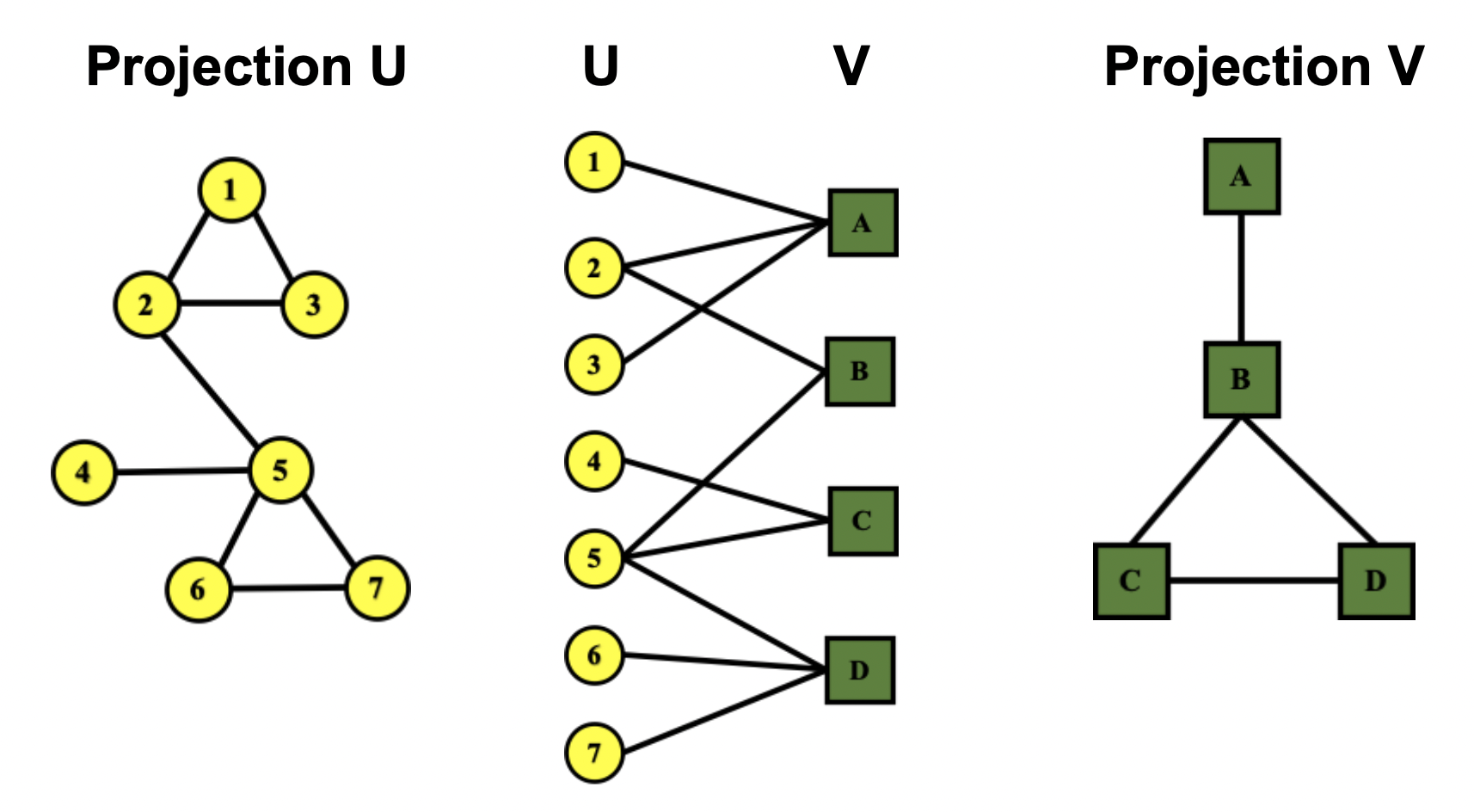
U-V 의 노드를 가지는 이분 그래프가 있다고 했을 때, 이를 Projection할 수 있음.

• Projection U : U노드가 1개 이상의 공통된 V와 연결되어 있으면 Projection graph U의 노드를 연결
  • Ex) 이분 그래프의 1번, 2번 노드가 노드 A와 공통적으로 연결되어 있으므로 Projection U graph의 1번-2번 노드를 연결
  • U가 저자, V가 논문이라면 Projection U graph는 한번이라도 같이 논문을 쓴 적 있는 사람들을 연결한 그래프가 된다.
• Projection V : V노드가 1개 이상의 공통된 U와 연결되어 있다면 Projection graph V의 노드를 연결
  • Ex) 이분 그래프의 A, B 노드가 노드 2와 공통적으로 연결되어 있으므로 Projection V graph의 A-B 노드를 연결
  • U가 저자, V가 논문이라면 Projection V graph는 같은 저자를 공유하는 논문을 연결한 그래프가 된다.

Representing Graphs

1) Adjacency Matrix

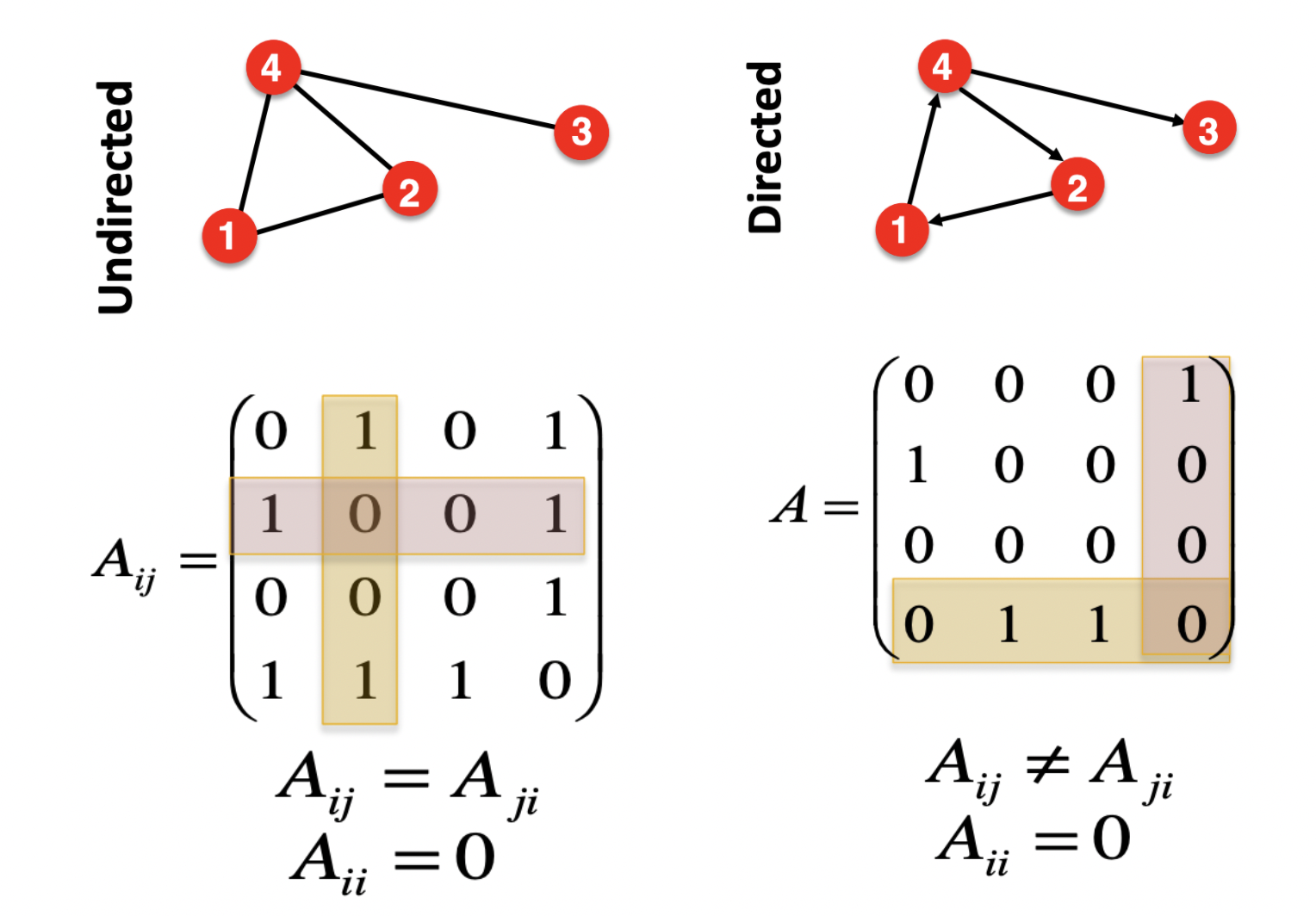
Undirected

• 방향성 없는 링크로 연결되어 있으므로,
  i→j , j→i 로의 경로가 모두 존재한다고 생각
  - $A_{ij}$ 와 $A_{ji}$ 모두 1로 표시
• Symmetric (대칭적)
• 🟨 : $k_i$ = $k_2$
• 🟥 : $k_j$= $k_2$
• 가로 sum = 세로 sum = degree
• 링크의 개수
  $L = \frac{1}{2} \sum^{N}_{i=1}{k_{i}} = \frac{1}{2} \sum^{N}_{i=1}{A_{ij}}$

Directed

• i → j 로 연결되어 있을 경우에 $A_{ij}$만 1로 표시
• Asymmetric (비대칭적)
• 🟨 : $k^{out}_i$ = $k^{out}_4$
• 🟥 : $k^{in}_j$ = $k^{in}_4$
• 가로 sum = out-degree
  세로 sum = in-degree
• 링크의 개수
  $L = \sum^{N}_{i=1}{k_{i}^{in}} = \sum^{N}_{i=1}{k_{i}^{out}} = \sum^{N}_{i,j}{A_{ij}}$

⚠️ Most real-world networks are sparse

$E << E_{max}$
$\bar{k} << N-1$ (= 한개의 노드가 최대로 가질 수 있는 엣지 수)

2) Edge list

• 연결된 엣지를 2차원 리스트로 저장 → DL Framework에서 많이 쓰임 !
  
• Graph manipulation / analysis (조작 및 분석)이 어려움
  • Ex) graph degree 계산이 어려움 등

⇒ 그래서 등장

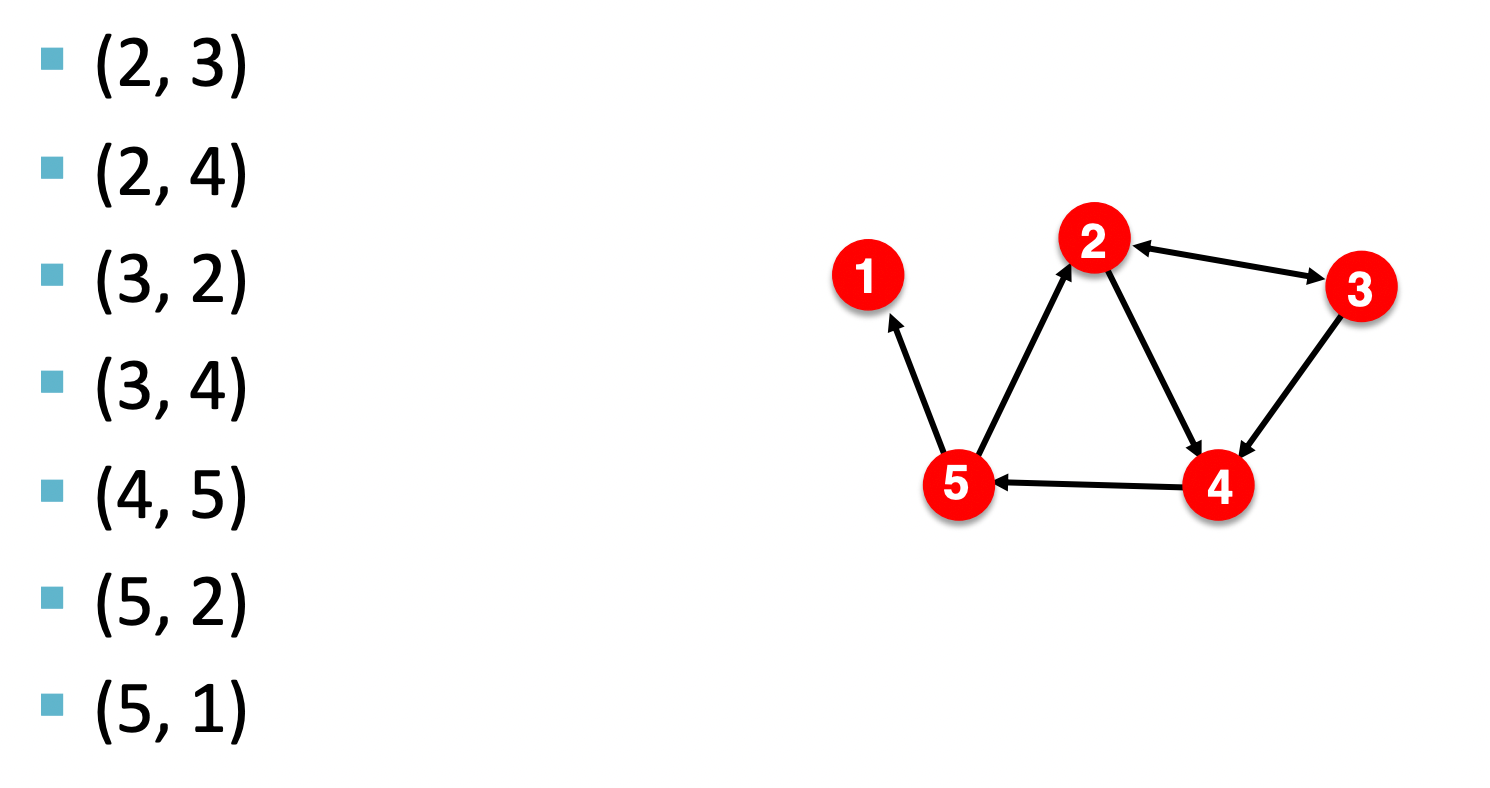
3) Adjancency list

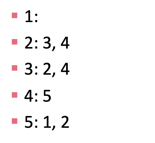
• Large & Sparse network를 다루기 용이
• 주어진 노드의 이웃을 빠르게 탐색 가능

cf > directed graph일땐 out-going과 in-going한 방향을 동시에 저장함.

More Types of Graphs

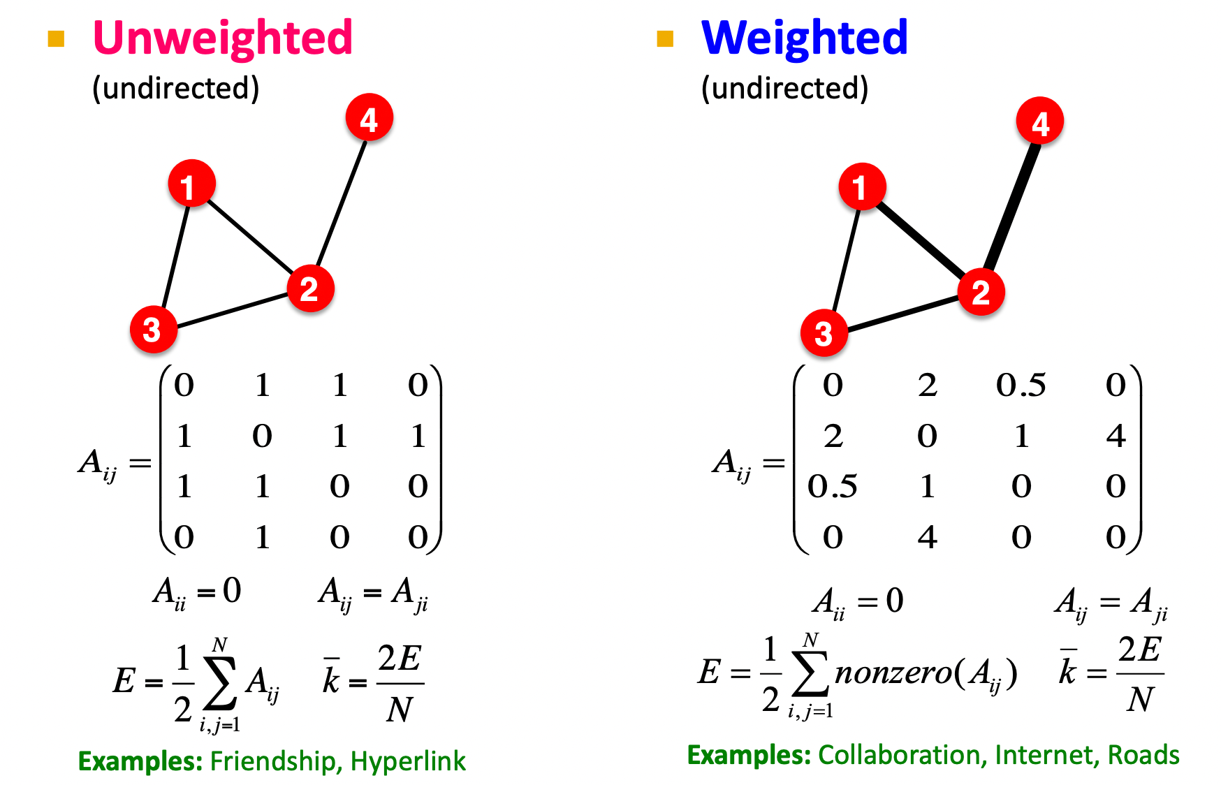
1) Unweighted vs. Weighted

2) Self-edges (self-loops) & Multigraph

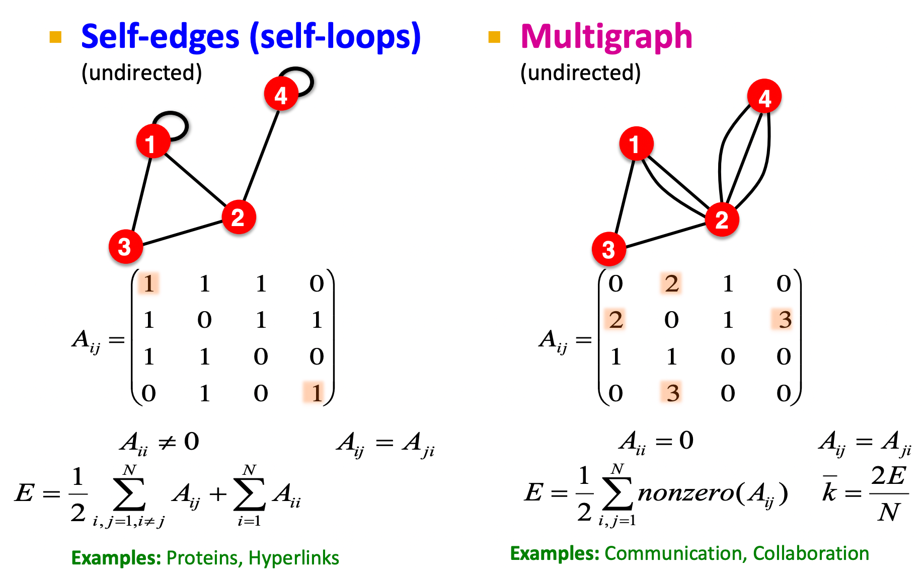
• matrix 대각선의 숫자가 0이 아님 = self-roof를 가짐을 의미
• node 4의 Degree = 3
• 가중치를 가지는 그래프와 비슷하게 표현됨
• weighted graph를 → multigraph로도 표현 가능

Notion of Connectivity

1. Undirected Graphs

Connected graph vs. Disconnected graph

• Connected : 모든 노드가 서로 연결 가능
• Disconnected : 2개 이상의 연결 요소로 구성
  • Largest Component: Giant Component
  • Isolated node (ex. node H)

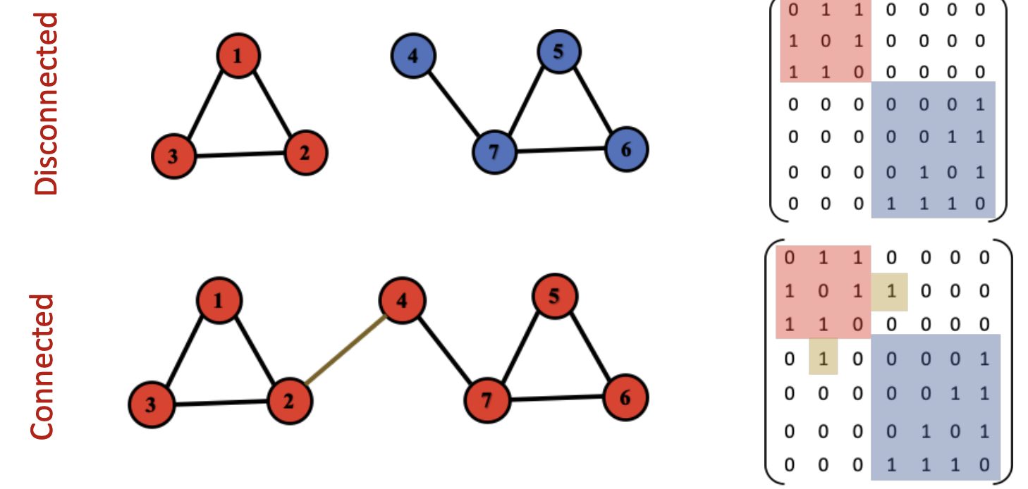
• Disconnected : 인접행렬이 대각선에 위치한 사각형 블록 형태로 나타남 → non-zero element가 블록 안에만 나타남

2. Directed Graphs

Strongly connected vs. Weakly connected

• 한 노드에서 다른 노드로 갈 수 있는 경로가 항상 존재함 → Strongly
• 방향을 무시하면 모두 연결되어 있음 But 일부 노드에서 다른 노드로 가는 경로가 존재하지 않음 → Weakly

Strongly connected components (SCCs)

: 강하게 연결된 연결된 노드의 집합 (방향 그래프의 부분집합)

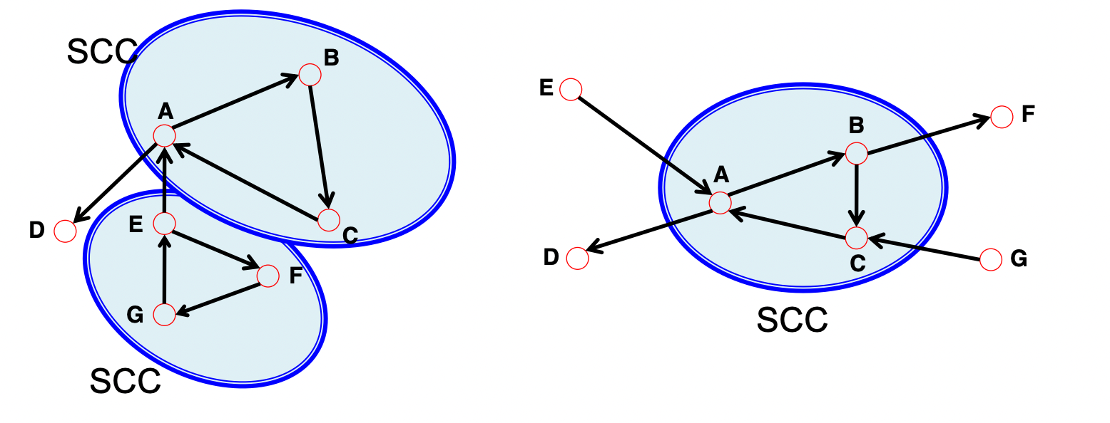
• In-component: nodes that can reach the SCC (ex. E of 2)
  Out-component: nodes that can be reached from the SCC (ex. D of 2)