케라스 공식문서
from tensorflow import keras
import numpy as np
import matplotlib.pyplot as plt
%matplotlib inline # 한글설정
1. 입력데이터
(1) 데이터 준비
x = np.arange(20)
y = x * 3 + 10
plt.plot(x,y)
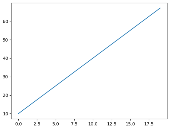
train을 위한 data로 x= 0, 1, 2, 3, ...., 19, y= 10, 13, 16, 19, ..., 67인 데이터를 준비했다.
이를 시각화하면 위와 같이 1차 함수가 그려진다.
x_test = np.arange(50,70)
y_test = x_test * 3 + 10
test를 위한 data로는 x= 50, 51, 52, ..., 69, y= 160, 163, 166, ..., 217인 데이터를 준비했다.
in_dim = 1
out_dim = 1
입력과 출력의 차원은 1로 설정했다.
2. 모델 구조 형성
Keras에서는 Sequential, Functional 방식으로 모델을 구현한다.
Sequential 방식은 모델에 필요한 layer들을 순차적으로 쌓는 방법이고, Functional 방식은 모델을 수식처럼 구현하는 방법이다.
두 방식 모두 함수 또는 클래스 형태로 만들 수 있다.
(1) Sequential 방식
def model_sequential(in_dim, out_dim):
	model = models.Sequential()
    model.add(layers.Dense(units=out_dim, input_shape=(in_dim,)))
    return model
함수 형태로 만드는 경우, models.Sequential()을 사용해 Sequential스타일로 진행한다고 설정한다.
이후 model.add()를 사용해 layer들을 쌓아주면 된다.
- layers.Dense: Fully Connected Layer 종류
- units: output 원소 개수
- input_shape: input 크기
- activation: activation 함수 설정
class modeling_sequential_class(models.Sequential):
    def __init__(self, in_dim, out_dim):
        self.in_dim = in_dim
        self.out_dim = out_dim
        super().__init__()
        self.add(layers.Dense(units =out_dim, input_shape=(in_dim,)))
클래스 형태로 만드는 경우. models.Sequential 을 상속받아 작성한다.
먼저 self.in_dim, self.out_dim으로 멤버 변수로 모델에 사용할 변수를 선언한다.
이후 super().__init__() 상속받은 Sequential 클래스를 초기화한 후에 모델에 레이어를 추가한다.
이때는 model.add()이 아닌 self.add()를 사용한다.
(2) Functional 방식
def modeling_functional(in_dim, out_dim):
    inputs = layers.Input(shape=(in_dim, ))
    y = layers.Dense(out_dim)(inputs)
    model = models.Model(inputs=inputs, outputs=y)
    return model
먼저 layers.Input(shape=(in_dim, ))으로 input layer를 정의한다. 이때 shape은 입력받는 벡터의 크기를 의미한다.
이후 layers.Dense(out_dim)(inputs)으로 layer를 쌓는다. 이전 layer인 input을 입력으로 받고, out_dim을 출력한다.
y = layers.Dense(out_dim)(inputs)을 계속 입력해서 모델 layer를 계속 쌓을 수 있다.
layer를 다 만들고 나면 models.Model(inputs=inputs, outputs=y)로 모델을 선언한다. 이때 입력과 출력을 인자로 입력한다.
class modeling_functional_class(models.Model):
    def __init__(self, in_dim, out_dim):
        self.in_dim = in_dim
        self.n_out = out_dim
        input = layers.Input(shape=(in_dim,))
        output = layers.Dense(out_dim)
        x = input
        y = output(x)
        super().__init__(x, y)
클래스 형식으로 모델을 만들때는 Sequential과 동일하게 self를 사용해 클래스 내에서 멤버 변수로 모델에 사용할 변수와 레이어를 선언한다.
x = input y = output(x)로 layer를 연결한다.
super().__init__(x, y)로 상속받은 모델의 클래스를 초기화한다.
(3) 모델 시각화
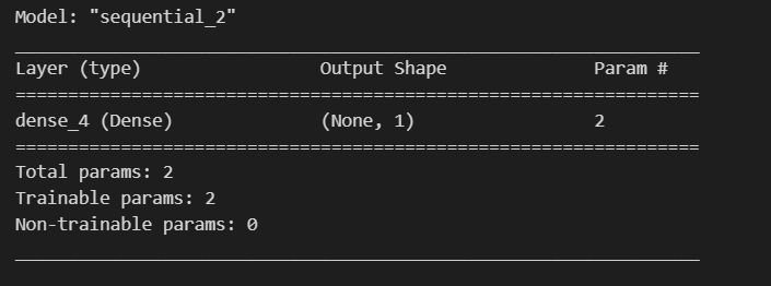
model.summary()나plot_model(model)을 사용한다.model.summary()가 좀더 간편하다.
model =  modeling_sequential(n_in, n_out)
model.summary()
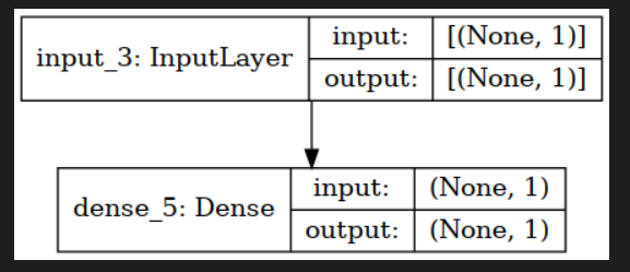
from tensorflow.keras.utils import plot_model
model =  modeling_functional(n_in, n_out)
plot_model(model, show_shapes=True)
3. 하이퍼파라미터 설정
- model.compile(loss, optimizer, metrics)
- loss(str): loss function(알고리즘이 예측한 값과 실제 답의 차이를 비교하기 위한 함수)
- 종류: binary_crossentropy, categorical_crossentropy, rmse, mse, mae, mape - optimizer(str): optimizer loss function의 최솟값을 찾고자 할때 사용할 알고리즘
- metrics(str): 검증 데이터에서의 학습 모델의 성능에 대한 평가지표
- 종류: loss, accuracy, top_k_categorical_accuracy, recall, precision, auc
- loss(str): loss function(알고리즘이 예측한 값과 실제 답의 차이를 비교하기 위한 함수)
model.compile(loss="mse", optimizer='sgd')
4. 모델 학습
- model.fit()
- x : 입력 데이터
- y : 입력 데이터의 Label
- batch_szie(int) : 데이터를 한번에 몇개를 입력할 것인지/size가 클수록 한번에 입력되는 data의 개수는 줄어든다.(train data/batch_size만큼 사용함)
- steps_per_epoch(int) : 전체 데이터셋을 몇 번 학습할지
- epochs(int) : Number of epochs to train the model
- verbose : 학습 출력 방식(0= silent, 1 = progress bar, 2 = one line per epoch)
- callbacks(list) : callback 함수
- validation_split(float) : train data 중 validation data로 사용될 비율
- validation_data : (x_val, y_val) 쌍으로 입력
- shuffle(bool) : 매 epoch 마다 데이터를 섞을지 여부
- history : 학습과정이 담겨있는 데이터 송출
history = model.fit(x, y, batch_size=5, epochs=100, validation_split=0.2)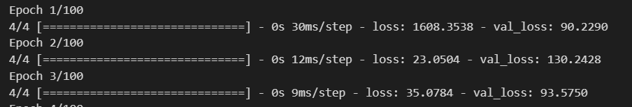
5. 모델 평가
- model.evaluate() : test 데이터에 대한 모델의 성능을 평가
- x : 입력 data (test data)
- y : 입력 data 의 Label
- batch_size(int) : 데이터를 한번에 몇개를 입력할 것인지/size가 클수록 한번에 입력되는 data의 개수는 줄어든다.(test data/batch_size만큼 사용함)
- steps(int) : 성능 계산을 위해 몇개의 batch를 test할 것인지
- verbose : 학습 출력 방식(0 = silent, 1 = progress bar, 2 = one line per epoch)
loss = model.evaluate(x_test, y_test, batch_size=20)
print('loss : %.4f'%(loss))

6. 모델 사용
- model.predict()
- x : 입력 data (test data)
- y : 입력 data 의 Label
- batch_size(int) : 데이터를 한번에 몇개를 입력할 것인지/size가 클수록 한번에 입력되는 data의 개수는 줄어든다.(test data/batch_size만큼 사용함)
- steps(int) : 성능 계산을 위해 몇개의 batch를 test할 것인지
- verbose : 학습 출력 방식(0 = silent, 1 = progress bar, 2 = one line per epoch)
new_x = np.arange(100, 120)
true_y = new_x * 3 + 10
test data를 먼저 만들어준다.
true_y는 위에서 만들었던 모델식을 사용해 만들면 된다.
pred_y = model.predict(new_x, batch_size=20, verbose = 0)
pred_y = np.reshape(pred_y,(-1,))
for y in zip(new_x, true_y, pred_y):
    print("x: %.2f,  y : %.2f,  y_predict : %.2f"%(y[0], y[1], y[2]))
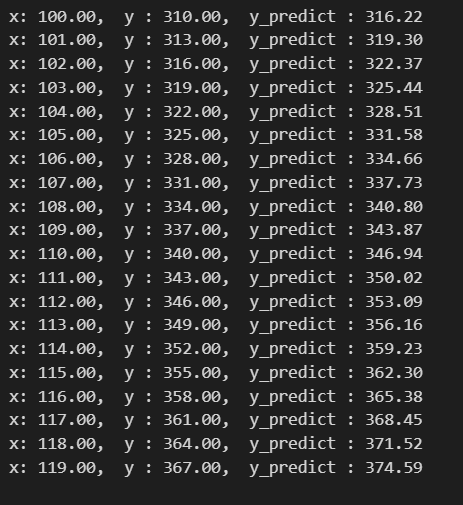
이제 train data를 FC모델에 넣고, 예측값을 출력해봤다.
꽤나 정답에 근사하게 예측하는 것을 볼 수 있다.
