NeRF 는 MLP 를 이용하여 3D scene 을 ray casting 으로 렌더링 하는 기법이다. 일반적인 Neural Network 가 generalization 능력을 극대화하는 방향으로 학습되는데 반면, NeRF 는 scene 을 하나의 non-linear function 이라고 간주하고 이를 MLP 로 근사한다. 즉, NeRF 에서 network 는 그 자체로 parameterized 된 scene 이다. 이때 network 는 좌표와 각도(i.e., ray)를 입력받아 그 ray 위 점들의 density 와 color 를 내뱉는다. scene 을 voxelize 하는 등의 방법 대신 continuous volumetric function 으로 표현하기 때문에 memory efficienct 하며, projected 2D images 를 input 으로 받기 때문에 3D voxel data 가 필요한 다른 방법 대비 training 도 효율적이다.
ECCV2020 Oral
1. Introduction
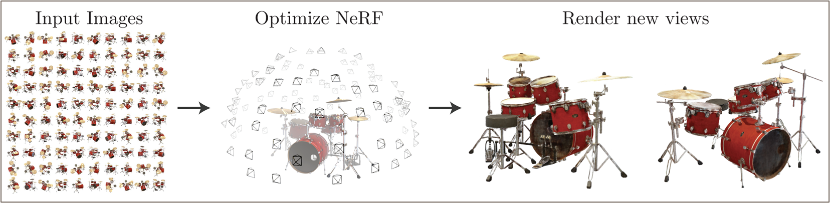
NeRF 의 기본적인 목표는 3D scene 을 implicit 하게 구성하는 MLP 를 이용하여 novel view 에 대한 projected image 를 구성하는 것이다. 현대 AI model 들이 training data 에 대한 commonality, 즉 pattern 을 representation 으로써 학습하는 representation learning 을 표방하는데 반면, NeRF 의 MLP 는 generalization 능력 대신 data sample 하나를 완전히 대변하는 역할을 한다. 즉 일종의 압축된 3D scene 으로써 MLP 를 이용한다.
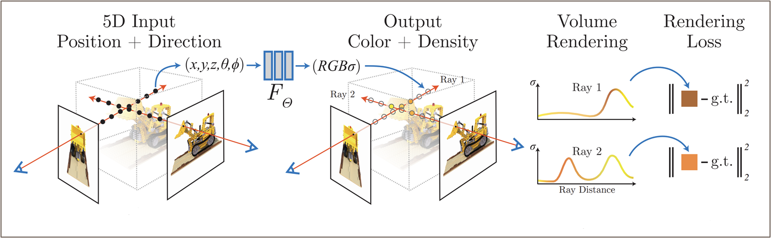
이때 이 MLP 는 다음과 같이 설계되는데,
- Input: location , direction
- Output: density , color
이는 NeRF 가 어떠한 특정한 방향 로 Scene 을 바라보았을 때, 그 Scene 의 특정 위치 가 어떠한 밀도, 색으로 로 나타내는지를 Accumulate 하여 scene 을 표현하기 때문이다.
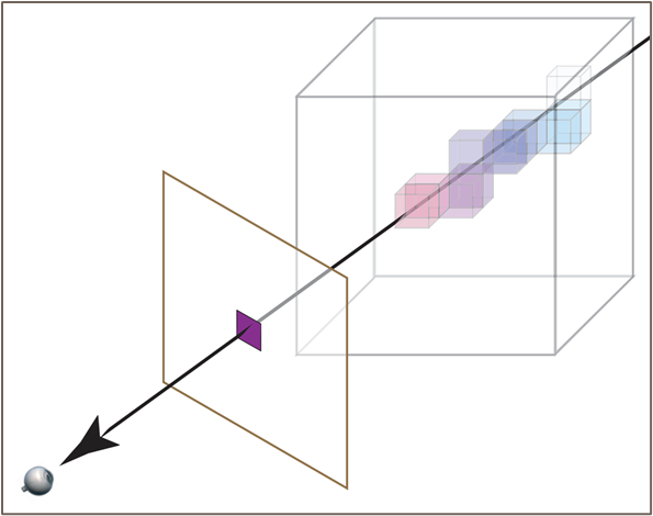
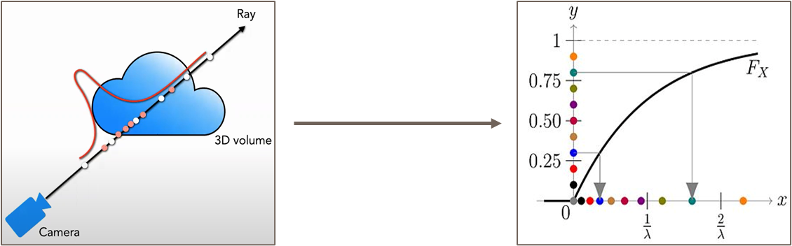
다음 그림과 같이 Projected image 의 한 좌표는 3d scene 에서의 한 직선 위의 수많은 location 들의 color 가 accumulated 되어 나타내게 된다.
NeRF 는 위와 같이 Scene 이 특정 방향으로 어떻게 projection 되는가를 이용해 novel view synthesis 를 구현한다. 이는 전통적인 volume ray casting 방식과 같은 방식이며, 이는 다음과 같은 장점을 갖는다.
- NeRF 의 학습은 projected direction 에 대한 GT 2D image 와의 MSE error 를 통해 학습되기 때문에 training 이 경제적이다.
- 3D scene 을 continuous volumetric function, 즉 MLP 로 표현하기 때문에 memory effifcient 하다.
2. Methods
2.1. Neural Radiance Fields
NeRF 는 다음과 같은 5d vector-valued function 으로 3D scene 을 나타낸다.
-
는 spherical coordinate 에서의 direction 을 나타내는데, 실제로 학습에는 3d cartessian unit vector 로 바꿔서 사용했다고 한다.
-
: differentiable probability of particle 로, input location 에 특정한 particle 이 있을 확률을 나타낸다. 즉 불투명도 (opacity) 를 대변하는 값이다.
-
c: 바라보는 방향 (direction) 에서 location 의 color 를 나타낸다. scene 을 바라보는 위치에 따라 illumination 이 달라져 color 가 바뀔 수 있으므로 (이를 non-lambertian effect 라고 한다), 이 값은 location 과 direction 에 모두 dependent 해야한다.
이는 일종의 빛 광선(Radiance)으로 공간을 구성하는 것과 같으므로, 이를 Radiance Fields 라고 한다. NeRF 는 이러한 Radiance Fields 를 MLP 로 구성하기 때문에 Neural Radiance Fields 인 셈.
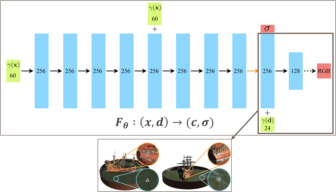
NeRF 의 MLP 는 위과 같은 9 fully-connected layers 를 갖는 MLP 로 구성된다.
-
density 는 direction 에 independent 하기 때문에 MLP 1st layer 에서 location 을 입력 받아 8th layer output 으로 예측된다 (scalar)
-
color 는 8th layer 의 feature 에 direction 까지 추가로 입력받아 도출된다.
( 는 input 에 대한 pre-processing encoding 함수이며, 아래에서 자세하게 설명하도록 한다 )
2.2. Volume Rendering with Radiance Fields
2.2.1 Continuous Volume Ray Casting
NeRF 는 상기 설명된 continuous volumetric function (MLP) 을 사용하여 volume ray casting 을 통해 volume rendering 을 진행한다. 이는 intro 에도 소개된 바와 같이, projected 된 2D image 를 통해 NeRF 를 학습하기 위함이다.
Volume Ray Casting 에서 어떠한 직선 를 따라 projected 된 한 점의 expected color 는 다음과 같이 정의할 수 있다.
-
: accumulated transmittance 로, 지점 앞까지의 ray 가 얼마나 투명했는지를 나타낸다. 즉 ray 가 current 앞에서 어떠한 particle 과도 만나지 않았을 경우 큰 값을 나타낸다.
-
: current 에서의 volume density 를 나타낸다. 즉, 현재 location 에서 어떠한 particle 이 있는지에 대한 값이다.
-
: 현재 location 에서 direction 을 고려한 color 이다.
즉 전체 적분은 Ray 를 따라서 opacity 가 높은 particle 의 color 를 많이 반영하고, opacity 가 낮은 입자의 color 는 적게 반영하여 estimated color 를 계산한다.
- 만약 어떠한 지점 앞에서 불투명한 입자를 만나게 된다면, accumulated transmittance 가 작아지게 되어, 불투명한 particle 뒤쪽의 color 는 거의 반영되지 않는다.
2.2.2. Discreatized Volume Ray Casting
상기 제시된 식을 approximation 하기 위해, 이를 Discreatization 하여 표현하면 다음과 같다.
-
로, discreate sampling 에서 adjacent sample 간의 거리이다. 즉 sampling 된 point 간의 거리가 너무 가까우면 비슷한 density 를 예측할 것이므로 이의 영향력을 줄여준다.
-
: current density 에 대해 를 고려해 를 취한 값이다. 는 small 에 대해서는 와 비슷한 monotonic increasing function 이며, large 에 대해서는 에 비해 더 완만한 gradient 를 그리게 된다.
-
즉 sampling 된 point 들간의 일종의 affine combination (-compositioning) 된 color 를 계산하게 된다.
기본적인 sampling rule 은 Stratified Sampling 을 따라 다음과 같이 정의된다.
이는 evenly spaced division 에서 각각 uniform sampling 하는 것으로, MLP 가 고정된 location set 에만 overfitting 되는 것을 방지한다.
2.3. Optimizing NeRF
2.3.1. Positional Encoding
NeRF 의 MLP 는 5d vector-valued function (실제로는 6d) 으로 표현되지만, 실제로 이렇게 학습하면 품질이 좋지 못하다고 한다.
이는 Neural Network 가 low frequency 에 biased 되기 쉽기 때문이며, 즉 high frequency 로 표현되는 fine detail 을 모사하기는 부족하다.
따라서 저자들은 MLP 의 input 으로 를 direct 하게 넣어주지 않고, high-dimensional space 로 mapping 하는 pre-processing 을 거쳐서 MLP 에 넣어주었다고 한다.
-
이는 Transformer 계열의 model 에서 spatial location 정보를 주기 위해 사용하는 positional encoding 과 동일한 형태이다.
-
positional encoding 은 relative position 을 가지는 feature 간의 관계를 쉽게 학습한다고 알려져 있다. (DETR Review)
2.3.2. Hierarchical Sampling
3D scene 안의 모든 점을 sampling 하는 것은 비효율적이기 때문에, 논문에서는 또한 2단계로 이루어진 Hierarchical Sampling 을 제시한다.
2.3.2.1. Coarse Network
NeRF 는 먼저 개의 점에 대해서 stratified sampling 을 이용하여 coarse sampling 을 진행한다.
이 때, coarse estimated color 은 실제 rendering 에 쓰이진 않는다. 대신, coarse network 의 output 은 efficient 하고 정밀한 discreatization 을 위한 sampling 으로 이용되게 된다.
2.3.2.2. Fine Network
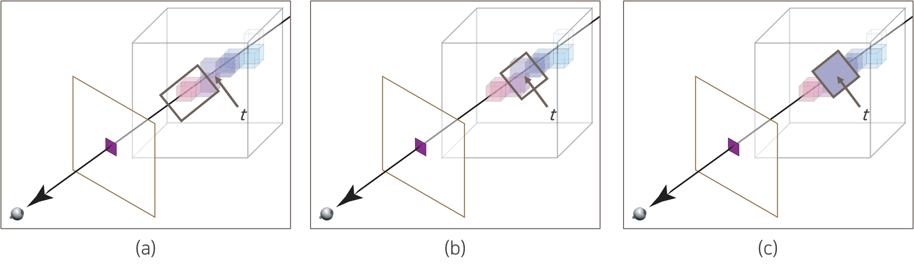
Fine Network 의 rendering 을 위해, 우선 Coarse network 를 통해 구한 를 normalize 하여 다음과 같은 piecewise constant PDF 를 구성한다.
이를 이용해 Inverse Transform Sampling 을 이용해 weight (i.e., opacity) 가 큰 구간에서 sampling 을 훨씬 정밀하게 진행한다.
이 과정을 시각적으로 표현하면 다음과 같다.
Fine Network 에서는 위의 sampling 을 이용하여 인 에 대한 Rendering 을 진행한다.
실제 구현엔 는 각각 로 사용되었다. 즉 NeRF 는 한 pixel 에 대해 총 192개의 점을 이용하여 rendering 되며, 이를 통한 2D GT image 와의 loss function 은 다음과 같이 정의된다.
Coasre Network 가 실제 rendering 엔 활용되지 않지만, 고품질의 결과물을 얻기 위하여 coarse, fine network 모두에 대해서 GT image 와 loss 를 계산하였다.
3. Normalized Device Coordinate
이 부분은 논문 본문에서는 자세히 다루지 않지만, NeRF 재구현을 위해서라면 필수적으로 알아야하는 부분이다. Computer Vision 에서 익숙하게 다루는 Homogeneous Coordinate 에 대해서 알아두는 편이 좋다.
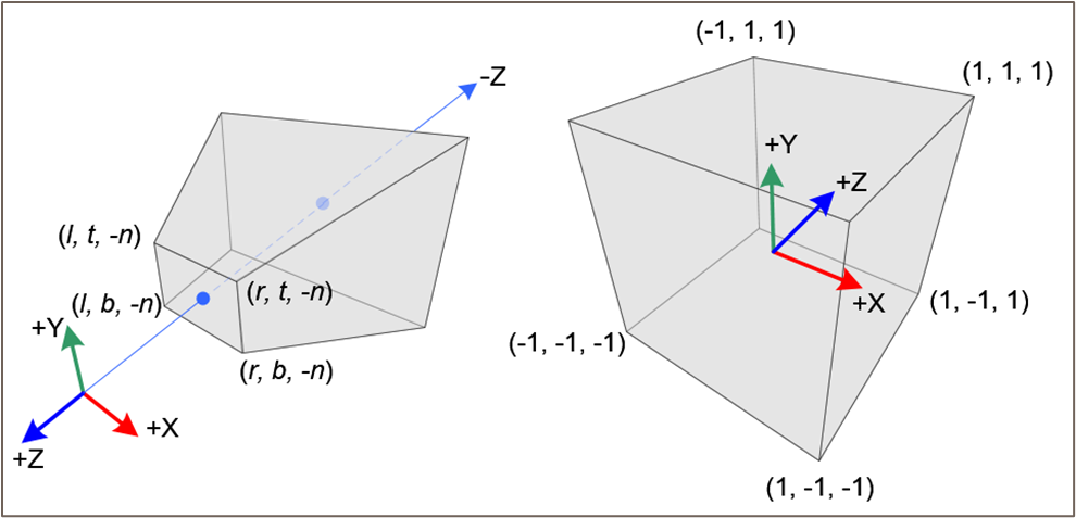
NeRF 의 이미지는, 일반적으로 COP 에서 World 를 관찰하는 unbounded Frustrum 형태이다 (그림 left). 이때 NeRF 의 MLP 는 input 으로 직접적인 3D coordinate 을 사용하기 때문에, 공간 전체를 효율적으로 표현할 방법이 필요하고, 그렇기 때문에 우리가 unbounded Frustrum 형태로 관찰한 real world 를 [-1, 1] 범위의 Normalized Device Coordinate (NDC) 로 바꿔줄 필요가 있다.
다시 말해 우리는 Unnormalized Real World Coordinate (보통 near, far plane 으로 범위를 제한) 를 NDC 로 mapping 하는 projection matrix 를 구해야 한다. 이러한 projection matrix M 은 다음과 같이 구할 수 있다.
-
coordinate 에 대해서는 각각 , , 로 변환하는 linear transformation 를 구한다.
-
coordinate 에 대해서 해당 linear transformation 은 가 나오게 되며, Frustrum 이 symmetric 임을 가정하기 때문에 이다.
-
에 대해서는 linear transformation 을 적용하지 않는데, 이는 depth 에 따라 occlusion 이 결정되므로 부동소수점 error 등이 일어날 경우 z-jittering 이 일어날 수 있기 때문이다. 따라서 가까운 object 에 대해서 가중치를 많이주는 형태의 non-linear transformation 을 취한다.
-
을 mapping 하는 해당 transformation 을 구하면 꼴이 나오게 된다.
-
이를 3D coordinate 에 대한 4D homogeneous coordinate projection matrix 로써 표현하게 되면 최종적으로 projection matrix M 의 형태는 다음과 같다.

실제 구현에서 이러한 NDC parameterization 은 llff 데이터 (forward-facing) 에만 적용되었다.
이는 전방위적으로 unbounded 인 world coordinate 의 경우 z-axis 에 대해서만 unbounded 인 NDC 로 적용했을 때 좋은 parameterization 방법이 아니기 때문이다.
이러한 NeRF 의 scene, ray parameterization 방법의 한계를 지적하는 NeRF++, Mip-NeRF 360 등의 후속 연구가 있으므로 다음에 다루도록 하겠다.
4. Experiments

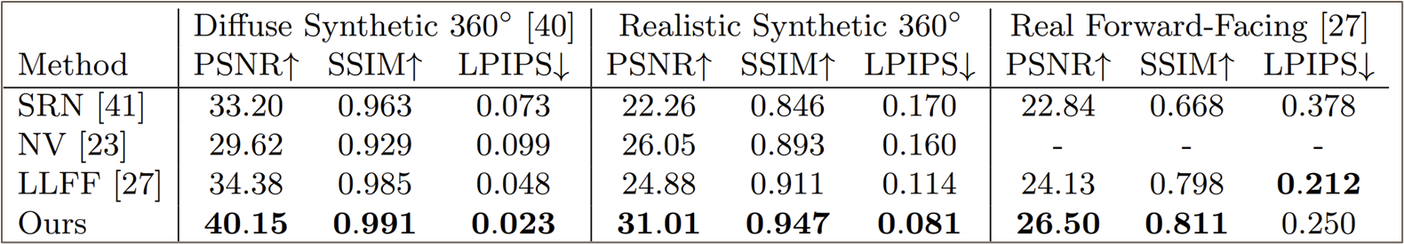
-
Generation 에 가까운 task 라 metric 으로 GAN 에서도 많이 쓰이는 PSNR 이나 SSIM 등을 사용한다.
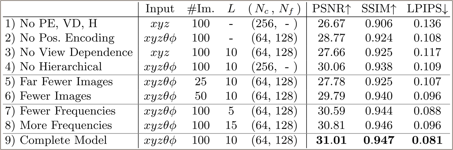
-
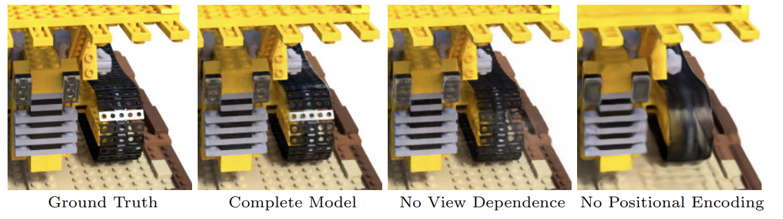
Albation Study 에서 positional encoding, view-dependency, hierarchical sampling 모두가 품질에 중요한 역할을 함을 알 수 있다.
You may also likes: