평가지표로는 RMSLE를 사용하자.
데이터 전처리
데이터 탐색 후 전처리를 진행하자
여러가지 전처리를 해보기 위해 원본 데이터는 따로 저장하고, 복사본을 사용하기
import warnings
warnings.filterwarnings('ignore')
import pandas as pd
import numpy as np
import seaborn as sns
import matplotlib.pyplot as plt

house_df_org = pd.read_csv('house_price.csv') # 원본을 저장해둠
house_df = house_df_org.copy() # 이걸로 처리
house_df.head(3)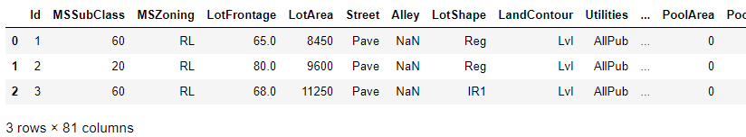
house_df.info()<class 'pandas.core.frame.DataFrame'>
RangeIndex: 1460 entries, 0 to 1459
Data columns (total 81 columns):
# Column Non-Null Count Dtype
--- ------ -------------- -----
0 Id 1460 non-null int64
1 MSSubClass 1460 non-null int64
2 MSZoning 1460 non-null object
3 LotFrontage 1201 non-null float64
4 LotArea 1460 non-null int64
5 Street 1460 non-null object
6 Alley 91 non-null object
7 LotShape 1460 non-null object
8 LandContour 1460 non-null object
9 Utilities 1460 non-null object
10 LotConfig 1460 non-null object
11 LandSlope 1460 non-null object
12 Neighborhood 1460 non-null object
13 Condition1 1460 non-null object
14 Condition2 1460 non-null object
15 BldgType 1460 non-null object
16 HouseStyle 1460 non-null object
17 OverallQual 1460 non-null int64
18 OverallCond 1460 non-null int64
19 YearBuilt 1460 non-null int64
20 YearRemodAdd 1460 non-null int64
21 RoofStyle 1460 non-null object
22 RoofMatl 1460 non-null object
23 Exterior1st 1460 non-null object
24 Exterior2nd 1460 non-null object
25 MasVnrType 1452 non-null object
26 MasVnrArea 1452 non-null float64
27 ExterQual 1460 non-null object
28 ExterCond 1460 non-null object
29 Foundation 1460 non-null object
30 BsmtQual 1423 non-null object
31 BsmtCond 1423 non-null object
32 BsmtExposure 1422 non-null object
33 BsmtFinType1 1423 non-null object
34 BsmtFinSF1 1460 non-null int64
35 BsmtFinType2 1422 non-null object
36 BsmtFinSF2 1460 non-null int64
37 BsmtUnfSF 1460 non-null int64
38 TotalBsmtSF 1460 non-null int64
39 Heating 1460 non-null object
40 HeatingQC 1460 non-null object
41 CentralAir 1460 non-null object
42 Electrical 1459 non-null object
43 1stFlrSF 1460 non-null int64
44 2ndFlrSF 1460 non-null int64
45 LowQualFinSF 1460 non-null int64
46 GrLivArea 1460 non-null int64
47 BsmtFullBath 1460 non-null int64
48 BsmtHalfBath 1460 non-null int64
49 FullBath 1460 non-null int64
50 HalfBath 1460 non-null int64
51 BedroomAbvGr 1460 non-null int64
52 KitchenAbvGr 1460 non-null int64
53 KitchenQual 1460 non-null object
54 TotRmsAbvGrd 1460 non-null int64
55 Functional 1460 non-null object
56 Fireplaces 1460 non-null int64
57 FireplaceQu 770 non-null object
58 GarageType 1379 non-null object
59 GarageYrBlt 1379 non-null float64
60 GarageFinish 1379 non-null object
61 GarageCars 1460 non-null int64
62 GarageArea 1460 non-null int64
63 GarageQual 1379 non-null object
64 GarageCond 1379 non-null object
65 PavedDrive 1460 non-null object
66 WoodDeckSF 1460 non-null int64
67 OpenPorchSF 1460 non-null int64
68 EnclosedPorch 1460 non-null int64
69 3SsnPorch 1460 non-null int64
70 ScreenPorch 1460 non-null int64
71 PoolArea 1460 non-null int64
72 PoolQC 7 non-null object
73 Fence 281 non-null object
74 MiscFeature 54 non-null object
75 MiscVal 1460 non-null int64
76 MoSold 1460 non-null int64
77 YrSold 1460 non-null int64
78 SaleType 1460 non-null object
79 SaleCondition 1460 non-null object
80 SalePrice 1460 non-null int64
dtypes: float64(3), int64(35), object(43)
memory usage: 924.0+ KB칼럼이 꽤 많고, null값이 존재하는 칼럼들 꽤 있다.
좀 더 구체적으로 알아보자
print('데이터 세트의 Shape:', house_df.shape)
print('\n전체 feature 들의 type \n',house_df.dtypes.value_counts())
isnull_series = house_df.isnull().sum()
print('\nNull 컬럼과 그 건수:\n ', isnull_series[isnull_series > 0].sort_values(ascending=False)) # Null이 1개 이상 있는 칼럼만 보기
데이터 세트의 Shape: (1460, 81)
전체 feature 들의 type
object 43
int64 35
float64 3
dtype: int64
Null 컬럼과 그 건수:
PoolQC 1453
MiscFeature 1406
Alley 1369
Fence 1179
FireplaceQu 690
LotFrontage 259
GarageYrBlt 81
GarageType 81
GarageFinish 81
GarageQual 81
GarageCond 81
BsmtFinType2 38
BsmtExposure 38
BsmtFinType1 37
BsmtCond 37
BsmtQual 37
MasVnrArea 8
MasVnrType 8
Electrical 1
dtype: int64object type도 꽤 많다. 이건 나중에 원핫인코딩 처리 해야할 듯
Null값이 대부분인 칼럼도 확인 됨
종속변수(Target)인 SalePrice의 분포도를 확인해보자
plt.title('Original Sale Price Histogram')
plt.xticks()
sns.histplot(house_df['SalePrice'], kde=True)
plt.show()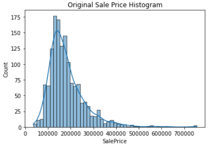
살짝 Right-skew 하다
log 변환하고 분포도를 확인해보자
plt.title('Log Transformed Sale Price Histogram')
log_SalePrice = np.log1p(house_df['SalePrice'])
sns.histplot(log_SalePrice, kde=True)
plt.show()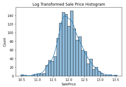
log 변환하니까 꽤 정규분포에 가까워졌다. 이걸 사용하도록 하자
우리는 평가지표로 RMSLE를 사용한다고 했다.
여기서 log 변환된 Target 값에 대해 RMSE를 구하면 그게 RMSLE가 됨!
Null을 가지는 칼럼을 Series로 뽑아내고,
dtypes를 출력해보자
null_column_count = house_df.isnull().sum()[house_df.isnull().sum() > 0]
house_df.dtypes[null_column_count.index]
LotFrontage float64
Alley object
MasVnrType object
MasVnrArea float64
BsmtQual object
BsmtCond object
BsmtExposure object
BsmtFinType1 object
BsmtFinType2 object
Electrical object
FireplaceQu object
GarageType object
GarageYrBlt float64
GarageFinish object
GarageQual object
GarageCond object
PoolQC object
Fence object
MiscFeature object
dtype: object
- SalePrice에 대해 log 변환 진행 (위에서는 그림만 그렸음)
- Null이 너무 많은 칼럼은 삭제
- 남은 수치형 칼럼은 평균값 대체
- 남은 object 칼럼 리스트를 출력
# SalePrice 로그 변환
# 두 번 돌리면 안 됨! 로그변환 한 것을 또 로그변환 해버림
original_SalePrice = house_df['SalePrice']
house_df['SalePrice'] = np.log1p(house_df['SalePrice'])

# Null 이 너무 많은 컬럼들과 불필요한 컬럼 삭제
house_df.drop(['Id','PoolQC' , 'MiscFeature', 'Alley', 'Fence','FireplaceQu'], axis=1 , inplace=True)
# Drop 하지 않는 숫자형 Null컬럼들은 평균값으로 대체
house_df.fillna(house_df.mean(),inplace=True)

# Null 값이 있는 피처명과 타입을 추출
null_column_count = house_df.isnull().sum()[house_df.isnull().sum() > 0]
print('## Null 피처의 Type :\n', house_df.dtypes[null_column_count.index])
## Null 피처의 Type :
MasVnrType object
BsmtQual object
BsmtCond object
BsmtExposure object
BsmtFinType1 object
BsmtFinType2 object
Electrical object
GarageType object
GarageFinish object
GarageQual object
GarageCond object
dtype: object원핫인코딩 수행한 데이터프레임을 house_df_ohe에 저장
print('get_dummies() 수행 전 데이터 Shape:', house_df.shape)
house_df_ohe = pd.get_dummies(house_df)
print('get_dummies() 수행 후 데이터 Shape:', house_df_ohe.shape)

null_column_count = house_df_ohe.isnull().sum()[house_df_ohe.isnull().sum() > 0]
print('## Null 피처의 Type :\n', house_df_ohe.dtypes[null_column_count.index])
get_dummies() 수행 전 데이터 Shape: (1460, 75)
get_dummies() 수행 후 데이터 Shape: (1460, 271)
## Null 피처의 Type :
Series([], dtype: object)선형 회귀 모델 학습/예측/평가
위에서 말한 것처럼 log 변환된 Target 값에 대해 RMSE를 구하면 그게 RMSLE가 됨!
여러 모델을 돌려볼 것이기 때문에 예측/평가는 함수로 만들어두고, 후에 학습만 개별적으로 진행하자
# 학습이 완료된 모델을 인자로 받아서 테스트 데이터로 예측하고 RMSE를 계산
def get_rmse(model):
    pred = model.predict(X_test)
    # y_test, pred는 로그 스케일임.
    mse = mean_squared_error(y_test , pred)
    rmse = np.sqrt(mse)
    print('{0} 로그 변환된 RMSE: {1}'.format(model.__class__.__name__,np.round(rmse, 3)))
    return rmse

# 여러 모델들을 list 형태로 인자로 받아서 개별 모델들의 RMSE를 list로 반환.
def get_rmses(models):
    rmses = [ ]
    for model in models:
        rmse = get_rmse(model)
        rmses.append(rmse)
    return rmses
Linear/Ridge/Lasso Regression 각각 학습 예측 평가 수행
from sklearn.linear_model import LinearRegression, Ridge, Lasso
from sklearn.model_selection import train_test_split
from sklearn.metrics import mean_squared_error

y_target = house_df_ohe['SalePrice']
X_features = house_df_ohe.drop('SalePrice',axis=1, inplace=False)

X_train, X_test, y_train, y_test = train_test_split(X_features, y_target, test_size=0.2, random_state=156)

# LinearRegression, Ridge, Lasso 학습, 예측, 평가
lr_reg = LinearRegression()
lr_reg.fit(X_train, y_train)

ridge_reg = Ridge()
ridge_reg.fit(X_train, y_train)

lasso_reg = Lasso()
lasso_reg.fit(X_train, y_train)

models = [lr_reg, ridge_reg, lasso_reg]
get_rmses(models)
LinearRegression 로그 변환된 RMSE: 0.132
Ridge 로그 변환된 RMSE: 0.128
Lasso 로그 변환된 RMSE: 0.176
[0.1318957657915436, 0.12750846334053045, 0.17628250556471395]Lasso가 좀 별로이고, Ridge가 제일 잘 나왔다.
각 회귀 계수를 시각화해보자 상위 10개, 하위 10개의 회귀 계수 값을 Series로 생성하는 함수 만들기
def get_top_bottom_coef(model):
    # coef_ 속성을 기반으로 Series 객체를 생성. index는 컬럼명.
    coef = pd.Series(model.coef_, index=X_features.columns)

    # + 상위 10개 , - 하위 10개 coefficient 추출하여 반환.
    coef_high = coef.sort_values(ascending=False).head(10)
    coef_low = coef.sort_values(ascending=False).tail(10)
    return coef_high, coef_low
세 가지 모델에 대해서 시각화 진행
def visualize_coefficient(models):
    # 3개 회귀 모델의 시각화를 위해 3개의 컬럼을 가지는 subplot 생성
    fig, axs = plt.subplots(figsize=(24,10),nrows=1, ncols=3)
    fig.tight_layout()
    # 입력인자로 받은 list객체인 models에서 차례로 model을 추출하여 회귀 계수 시각화.
    for i_num, model in enumerate(models):
        # 상위 10개, 하위 10개 회귀 계수를 구하고, 이를 판다스 concat으로 결합.
        coef_high, coef_low = get_top_bottom_coef(model)
        coef_concat = pd.concat( [coef_high , coef_low] )
        # 순차적으로 ax subplot에 barchar로 표현. 한 화면에 표현하기 위해 tick label 위치와 font 크기 조정.
        axs[i_num].set_title(model.__class__.__name__+' Coeffiecents', size=25)
        axs[i_num].tick_params(axis="y",direction="in", pad=-120)
        for label in (axs[i_num].get_xticklabels() + axs[i_num].get_yticklabels()):
            label.set_fontsize(22)
        sns.barplot(x=coef_concat.values, y=coef_concat.index , ax=axs[i_num])

# 앞 예제에서 학습한 lr_reg, ridge_reg, lasso_reg 모델의 회귀 계수 시각화.
models = [lr_reg, ridge_reg, lasso_reg]
visualize_coefficient(models)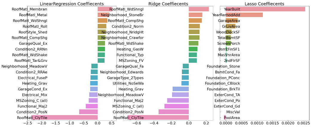
전체에 대해서 교차 검증을 진행
타겟값을 로그 변환 했으니까 실제로는 RMSLE를 구한 것임
from sklearn.model_selection import cross_val_score

def get_avg_rmse_cv(models):
    for model in models:
        # 분할하지 않고 전체 데이터로 cross_val_score( ) 수행. 모델별 CV RMSE값과 평균 RMSE 출력
        rmse_list = np.sqrt(-cross_val_score(model, X_features, y_target,
                                             scoring="neg_mean_squared_error", cv = 5))
        rmse_avg = np.mean(rmse_list)
        print('\n{0} CV RMSE 값 리스트: {1}'.format( model.__class__.__name__, np.round(rmse_list, 3)))
        print('{0} CV 평균 RMSE 값: {1}'.format( model.__class__.__name__, np.round(rmse_avg, 3)))

# 앞 예제에서 학습한 ridge_reg, lasso_reg 모델의 CV RMSE값 출력
models = [ridge_reg, lasso_reg]
get_avg_rmse_cv(models)
Ridge CV RMSE 값 리스트: [0.117 0.154 0.142 0.117 0.189]
Ridge CV 평균 RMSE 값: 0.144
Lasso CV RMSE 값 리스트: [0.161 0.204 0.177 0.181 0.265]
Lasso CV 평균 RMSE 값: 0.198Ridge가 좀 더 우수한 성능을 보인다.
alpha값을 변겨해 하면서 그리드서치 진행
from sklearn.model_selection import GridSearchCV

def print_best_params(model, params):
    grid_model = GridSearchCV(model, param_grid=params,
                              scoring='neg_mean_squared_error', cv=5)
    grid_model.fit(X_features, y_target)
    rmse = np.sqrt(-1* grid_model.best_score_)
    print('{0} 5 CV 시 최적 평균 RMSE 값: {1}, 최적 alpha:{2}'.format(model.__class__.__name__,
                                        np.round(rmse, 4), grid_model.best_params_))
    return grid_model.best_estimator_

ridge_params = { 'alpha':[0.05, 0.1, 1, 5, 8, 10, 12, 15, 20] }
lasso_params = { 'alpha':[0.001, 0.005, 0.008, 0.05, 0.03, 0.1, 0.5, 1,5, 10] }
best_rige = print_best_params(ridge_reg, ridge_params)
best_lasso = print_best_params(lasso_reg, lasso_params)
Ridge 5 CV 시 최적 평균 RMSE 값: 0.1418, 최적 alpha:{'alpha': 12}
Lasso 5 CV 시 최적 평균 RMSE 값: 0.142, 최적 alpha:{'alpha': 0.001}그리드 서치 진행해보니 둘이 거의 유사하다.
각각 최적화된 alpha 값으로 학습 데이터과 테스트 데이터로 예측 및 평가를 수행하고, 회귀 계수 시각화까지 진행
# 앞의 최적화 alpha값으로 학습데이터로 학습, 테스트 데이터로 예측 및 평가 수행.
lr_reg = LinearRegression()
lr_reg.fit(X_train, y_train)

ridge_reg = Ridge(alpha=12)
ridge_reg.fit(X_train, y_train)

lasso_reg = Lasso(alpha=0.001)
lasso_reg.fit(X_train, y_train)

# 모든 모델의 RMSE 출력
models = [lr_reg, ridge_reg, lasso_reg]
get_rmses(models)

# 모든 모델의 회귀 계수 시각화
models = [lr_reg, ridge_reg, lasso_reg]
visualize_coefficient(models)
LinearRegression 로그 변환된 RMSE: 0.132
Ridge 로그 변환된 RMSE: 0.124
Lasso 로그 변환된 RMSE: 0.12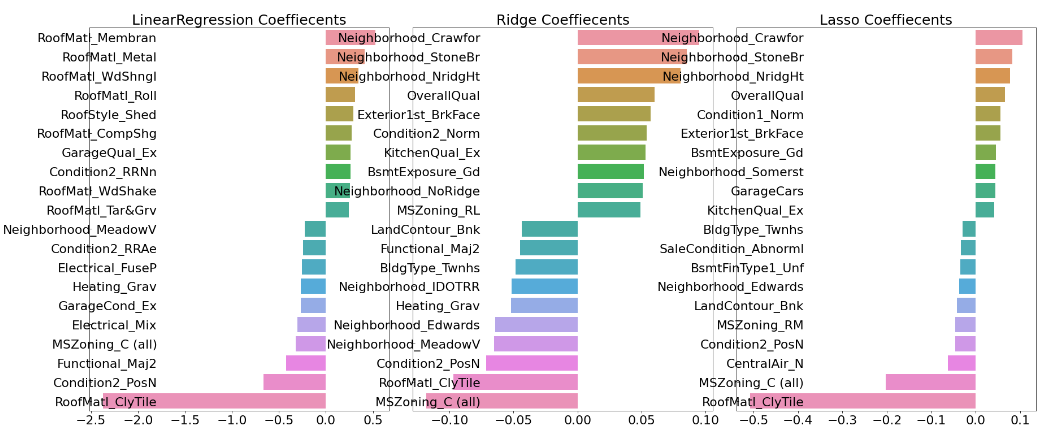
object가 아닌 칼럼 (수치형 칼럼)에 대해 skew 정도를 확인해보자
skew가 1이 넘는 칼럼들만 출력
from scipy.stats import skew

# object가 아닌 숫자형 피쳐의 컬럼 index 객체 추출.
features_index = house_df.dtypes[house_df.dtypes != 'object'].index
# house_df에 컬럼 index를 [ ]로 입력하면 해당하는 컬럼 데이터 셋 반환. apply lambda로 skew( )호출
skew_features = house_df[features_index].apply(lambda x : skew(x))
# skew 정도가 1 이상인 컬럼들만 추출.
skew_features_top = skew_features[skew_features > 1]
print(skew_features_top.sort_values(ascending=False))
MiscVal 24.451640
PoolArea 14.813135
LotArea 12.195142
3SsnPorch 10.293752
LowQualFinSF 9.002080
KitchenAbvGr 4.483784
BsmtFinSF2 4.250888
ScreenPorch 4.117977
BsmtHalfBath 4.099186
EnclosedPorch 3.086696
MasVnrArea 2.673661
LotFrontage 2.382499
OpenPorchSF 2.361912
BsmtFinSF1 1.683771
WoodDeckSF 1.539792
TotalBsmtSF 1.522688
MSSubClass 1.406210
1stFlrSF 1.375342
GrLivArea 1.365156
dtype: float64skew가 1보다 큰 칼럼들에 대해 log 변환을 적용하고, 다시 하이퍼 파라미터 튜닝 후 학습/예측/평가 해보자
house_df[skew_features_top.index] = np.log1p(house_df[skew_features_top.index])# Skew가 높은 피처들을 로그 변환 했으므로 다시 원-핫 인코딩 적용 및 피처/타겟 데이터 셋 생성,
house_df_ohe = pd.get_dummies(house_df)
y_target = house_df_ohe['SalePrice']
X_features = house_df_ohe.drop('SalePrice',axis=1, inplace=False)
X_train, X_test, y_train, y_test = train_test_split(X_features, y_target, test_size=0.2, random_state=156)
# 피처들을 로그 변환 후 다시 최적 하이퍼 파라미터와 RMSE 출력
ridge_params = { 'alpha':[0.05, 0.1, 1, 5, 8, 10, 12, 15, 20] }
lasso_params = { 'alpha':[0.001, 0.005, 0.008, 0.05, 0.03, 0.1, 0.5, 1,5, 10] }
best_ridge = print_best_params(ridge_reg, ridge_params)
best_lasso = print_best_params(lasso_reg, lasso_params)Ridge 5 CV 시 최적 평균 RMSE 값: 0.1275, 최적 alpha:{'alpha': 10}
Lasso 5 CV 시 최적 평균 RMSE 값: 0.1252, 최적 alpha:{'alpha': 0.001# 앞의 최적화 alpha값으로 학습데이터로 학습, 테스트 데이터로 예측 및 평가 수행.
lr_reg = LinearRegression()
lr_reg.fit(X_train, y_train)
ridge_reg = Ridge(alpha=10)
ridge_reg.fit(X_train, y_train)
lasso_reg = Lasso(alpha=0.001)
lasso_reg.fit(X_train, y_train)
# 모든 모델의 RMSE 출력
models = [lr_reg, ridge_reg, lasso_reg]
get_rmses(models)
# 모든 모델의 회귀 계수 시각화
models = [lr_reg, ridge_reg, lasso_reg]
visualize_coefficient(models)LinearRegression 로그 변환된 RMSE: 0.128
Ridge 로그 변환된 RMSE: 0.122
Lasso 로그 변환된 RMSE: 0.119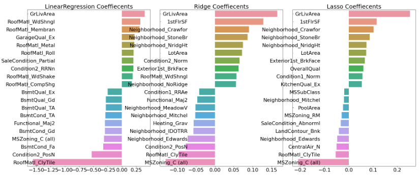
성능 향상이 조금 있었다.
이제 이상치 처리를 진행하자
회귀 계수가 높아서 주요 Feature로 확인 되는 GrLivArea에 대해 산점도를 나타내자
plt.scatter(x = house_df_org['GrLivArea'], y = house_df_org['SalePrice'])
plt.ylabel('SalePrice', fontsize=15)
plt.xlabel('GrLivArea', fontsize=15)
plt.show()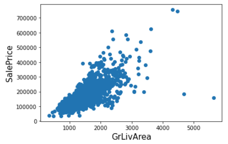
GrLivArea와 SalePrice에 대해서 log 변환을 고려한 조건을 지정해서, 이상치를 제거하자
# GrLivArea와 SalePrice 모두 로그 변환되었으므로 이를 반영한 조건 생성.
cond1 = house_df_ohe['GrLivArea'] > np.log1p(4000)
cond2 = house_df_ohe['SalePrice'] < np.log1p(500000)
outlier_index = house_df_ohe[cond1 & cond2].index

print('아웃라이어 레코드 index :', outlier_index.values)
print('아웃라이어 삭제 전 house_df_ohe shape:', house_df_ohe.shape)
# DataFrame의 index를 이용하여 아웃라이어 레코드 삭제.
house_df_ohe.drop(outlier_index , axis=0, inplace=True)
print('아웃라이어 삭제 후 house_df_ohe shape:', house_df_ohe.shape)
아웃라이어 레코드 index : [ 523 1298]
아웃라이어 삭제 전 house_df_ohe shape: (1460, 271)
아웃라이어 삭제 후 house_df_ohe shape: (1458, 271)2개의 행이 제거된 것으로 확인 된다.
이상치를 제거할 때는 행을 제거하니까axis=0인 것을 잊지 말기
이상치 제거 후 다시 그리드 서치를 진행하자!
y_target = house_df_ohe['SalePrice']
X_features = house_df_ohe.drop('SalePrice',axis=1, inplace=False)
X_train, X_test, y_train, y_test = train_test_split(X_features, y_target, test_size=0.2, random_state=156)

ridge_params = { 'alpha':[0.05, 0.1, 1, 5, 8, 10, 12, 15, 20] }
lasso_params = { 'alpha':[0.001, 0.005, 0.008, 0.05, 0.03, 0.1, 0.5, 1,5, 10] }
best_ridge = print_best_params(ridge_reg, ridge_params)
best_lasso = print_best_params(lasso_reg, lasso_params)
Ridge 5 CV 시 최적 평균 RMSE 값: 0.1125, 최적 alpha:{'alpha': 8}
Lasso 5 CV 시 최적 평균 RMSE 값: 0.1122, 최적 alpha:{'alpha': 0.001}# 앞의 최적화 alpha값으로 학습데이터로 학습, 테스트 데이터로 예측 및 평가 수행.
lr_reg = LinearRegression()
lr_reg.fit(X_train, y_train)
ridge_reg = Ridge(alpha=8)
ridge_reg.fit(X_train, y_train)
lasso_reg = Lasso(alpha=0.001)
lasso_reg.fit(X_train, y_train)
# 모든 모델의 RMSE 출력
models = [lr_reg, ridge_reg, lasso_reg]
get_rmses(models)
# 모든 모델의 회귀 계수 시각화
models = [lr_reg, ridge_reg, lasso_reg]
visualize_coefficient(models)LinearRegression 로그 변환된 RMSE: 0.129
Ridge 로그 변환된 RMSE: 0.103
Lasso 로그 변환된 RMSE: 0.1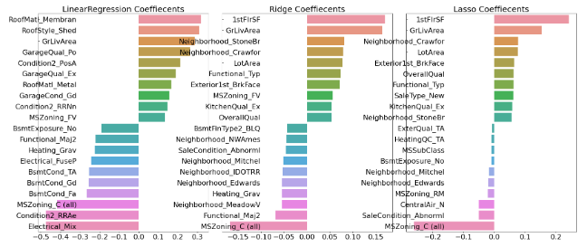
역시 이상치만 잘 제거해도 성능이 꽤 향상 된다.
하지만 이상치 처리는 테스트 데이터에도 이런 데이터가 있을지를 잘 고려해야한다.
최대한 보수적으로 진행!
처리 후 GrLivArea의 회귀 계수가 조금 조정된 듯 보인다.
회귀 트리 계열 학습/예측/평가
이번엔 트리 계열 모델인 XGBoost와 LightGBM을 사용하자
학습 시간 관계상 각각n_estimators=1000으로만 설정하고 교차 검증을 진행
->print_best_parmas()를 사용하지만 실제로는 파라미터 하나 뿐
from xgboost import XGBRegressor

xgb_params = {'n_estimators':[1000]}
xgb_reg = XGBRegressor(n_estimators=1000, learning_rate=0.05,
                       colsample_bytree=0.5, subsample=0.8)
best_xgb = print_best_params(xgb_reg, xgb_params)
XGBRegressor 5 CV 시 최적 평균 RMSE 값: 0.1178, 최적 alpha:{'n_estimators': 1000}from lightgbm import LGBMRegressor
lgbm_params = {'n_estimators':[1000]}
lgbm_reg = LGBMRegressor(n_estimators=1000, learning_rate=0.05, num_leaves=4,
subsample=0.6, colsample_bytree=0.4, reg_lambda=10, n_jobs=-1)
best_lgbm = print_best_params(lgbm_reg, lgbm_params)LGBMRegressor 5 CV 시 최적 평균 RMSE 값: 0.1163, 최적 alpha:{'n_estimators': 1000}각각 Feature Importance를 시각화하자
# 모델의 중요도 상위 20개의 피처명과 그때의 중요도값을 Series로 반환.
def get_top_features(model):
    ftr_importances_values = model.feature_importances_
    ftr_importances = pd.Series(ftr_importances_values, index=X_features.columns  )
    ftr_top20 = ftr_importances.sort_values(ascending=False)[:20]
    return ftr_top20

def visualize_ftr_importances(models):
    # 2개 회귀 모델의 시각화를 위해 2개의 컬럼을 가지는 subplot 생성
    fig, axs = plt.subplots(figsize=(24,10),nrows=1, ncols=2)
    fig.tight_layout()
    # 입력인자로 받은 list객체인 models에서 차례로 model을 추출하여 피처 중요도 시각화.
    for i_num, model in enumerate(models):
        # 중요도 상위 20개의 피처명과 그때의 중요도값 추출
        ftr_top20 = get_top_features(model)
        axs[i_num].set_title(model.__class__.__name__+' Feature Importances', size=25)
        #font 크기 조정.
        for label in (axs[i_num].get_xticklabels() + axs[i_num].get_yticklabels()):
            label.set_fontsize(22)
        sns.barplot(x=ftr_top20.values, y=ftr_top20.index , ax=axs[i_num])

# 앞 예제에서 print_best_params( )가 반환한 GridSearchCV로 최적화된 모델의 피처 중요도 시각화
models = [best_xgb, best_lgbm]
visualize_ftr_importances(models)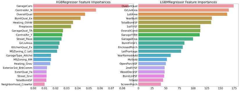
혼합 예측
앙상블과 비슷한 것으로 생각하면 됨
estimator.predict(test)한 것을 가중 평균을 내면 됨!
여기서는0.4 * ridge_pred + 0.6 * lasso_pred로 고정했는데,
실제로는 가중치를 바꿔가면서 성능이 좋은 것을 선택!
def get_rmse_pred(preds):
    for key in preds.keys():
        pred_value = preds[key]
        mse = mean_squared_error(y_test , pred_value)
        rmse = np.sqrt(mse)
        print('{0} 모델의 RMSE: {1}'.format(key, rmse))

# 개별 모델의 학습
ridge_reg = Ridge(alpha=8)
ridge_reg.fit(X_train, y_train)
lasso_reg = Lasso(alpha=0.001)
lasso_reg.fit(X_train, y_train)
# 개별 모델 예측
ridge_pred = ridge_reg.predict(X_test)
lasso_pred = lasso_reg.predict(X_test)

# 개별 모델 예측값 혼합으로 최종 예측값 도출
pred = 0.4 * ridge_pred + 0.6 * lasso_pred
preds = {'최종 혼합': pred,
         'Ridge': ridge_pred,
         'Lasso': lasso_pred}
#최종 혼합 모델, 개별모델의 RMSE 값 출력
get_rmse_pred(preds)
최종 혼합 모델의 RMSE: 0.10007930884470519
Ridge 모델의 RMSE: 0.10345177546603272
Lasso 모델의 RMSE: 0.10024170460890039xgb_reg = XGBRegressor(n_estimators=1000, learning_rate=0.05,
colsample_bytree=0.5, subsample=0.8)
lgbm_reg = LGBMRegressor(n_estimators=1000, learning_rate=0.05, num_leaves=4,
subsample=0.6, colsample_bytree=0.4, reg_lambda=10, n_jobs=-1)
xgb_reg.fit(X_train, y_train)
lgbm_reg.fit(X_train, y_train)
xgb_pred = xgb_reg.predict(X_test)
lgbm_pred = lgbm_reg.predict(X_test)
pred = 0.5 * xgb_pred + 0.5 * lgbm_pred
preds = {'최종 혼합': pred,
'XGBM': xgb_pred,
'LGBM': lgbm_pred}
get_rmse_pred(preds)최종 혼합 모델의 RMSE: 0.10170077353447762
XGBM 모델의 RMSE: 0.10738295638346222
LGBM 모델의 RMSE: 0.10382510019327311스태킹 모델을 이용한 예측
스태킹 먼저 작성 후 나머지 작성