[ML] 차원 축소 - SVD (Singular Value Decomposition)

SVD 개요

SVD, Singular Value Decomposition, 특이값 분해

---

고윳값 분해와 비교

앞에서 배운 고윳값 분해와 비교해보자


고윳값 분해

• 정방행렬만 고유벡터로 분해
• PCA는 분해된 고유벡터에 원본 데이터를 투영하여 차원 축소

특이값 분해 (SVD)

• 정방행렬뿐만 아니라 행과 열의 크기가 다른 $m$ x $n$ 분해도 가능
• $U$: 왼쪽 직교행렬
• $V$: 오른쪽 직교행렬
• $\Sigma$: 대각 행렬 (행렬의 대각 외의 나머지가 다 0)
• $U^TU = I$, $V^TV = I$
• $\Sigma$의 대각에 위치한 값이 행렬 A의 특이값

---

SVD 유형

Full SVD

• 기본

Compact SVD

• 비대각 부분과 대각 원소가 0인 부분을 제거

Truncated SVD

• 대각 원소 가운데 상위 r 개만 추출하여 차원 축소
• 차원 축소 행렬 분해된 후 다시 분해된 행렬을 이용하여 원복된 데이터는 잡음이 제거된 형태로 재구성 됨

scikit-learn에서는 Truncated SVD로 차원 축소할 때 원본 데이터에 $U \Sigma$를 적용하여 차원 축소

---

SVD 활용

• 추천 엔진
• 문서의 잠재 의미 분석
• 이미지 압축/변환
• 의사(pseudo) 역행렬을 통한 모델 예측

---

SVD 실습

NumPy 에서 SVD를 지원한다.
이건 기본 SVD임
랜덤 행렬을 하나 만들자

# numpy의 svd 모듈 import
import numpy as np
from numpy.linalg import svd

# 4X4 Random 행렬 a 생성 
np.random.seed(121)
a = np.random.randn(4,4)
print(np.round(a, 3))

[[-0.212 -0.285 -0.574 -0.44 ]
 [-0.33   1.184  1.615  0.367]
 [-0.014  0.63   1.71  -1.327]
 [ 0.402 -0.191  1.404 -1.969]]

SVD 행렬 분해 진행

U, Sigma, Vt = svd(a)
print(U.shape, Sigma.shape, Vt.shape)
print('U matrix:\n',np.round(U, 3))
print('Sigma Value:\n',np.round(Sigma, 3))
print('V transpose matrix:\n',np.round(Vt, 3))

(4, 4) (4,) (4, 4)
U matrix:
 [[-0.079 -0.318  0.867  0.376]
 [ 0.383  0.787  0.12   0.469]
 [ 0.656  0.022  0.357 -0.664]
 [ 0.645 -0.529 -0.328  0.444]]
Sigma Value:
 [3.423 2.023 0.463 0.079]
V transpose matrix:
 [[ 0.041  0.224  0.786 -0.574]
 [-0.2    0.562  0.37   0.712]
 [-0.778  0.395 -0.333 -0.357]
 [-0.593 -0.692  0.366  0.189]]

분해한 행렬을 다시 합쳐보자

 # Sigma를 다시 0 을 포함한 대칭행렬로 변환
Sigma_mat = np.diag(Sigma)
a_ = np.dot(np.dot(U, Sigma_mat), Vt)

print(Sigma_mat)
print(np.round(a_, 3))

[[3.4229581  0.         0.         0.        ]
 [0.         2.02287339 0.         0.        ]
 [0.         0.         0.46263157 0.        ]
 [0.         0.         0.         0.07935069]]
[[-0.212 -0.285 -0.574 -0.44 ]
 [-0.33   1.184  1.615  0.367]
 [-0.014  0.63   1.71  -1.327]
 [ 0.402 -0.191  1.404 -1.969]]

이번엔 Compact SVD를 실습해보자
데이터 의존도가 높은 원본 데이터 행렬을 생성하자
$4$ x $4$ 행렬인데, $rank$가 2인 행렬이다.

a[2] = a[0] + a[1]
a[3] = a[0]
print(np.round(a,3))

[[-0.212 -0.285 -0.574 -0.44 ]
 [-0.33   1.184  1.615  0.367]
 [-0.542  0.899  1.041 -0.073]
 [-0.212 -0.285 -0.574 -0.44 ]]

그냥 SVD 실행

U, Sigma, Vt = svd(a)
print(U.shape, Sigma.shape, Vt.shape)
print('Sigma Value:\n',np.round(Sigma,3))

(4, 4) (4,) (4, 4)
Sigma Value:
 [2.663 0.807 0.    0.   ]

0인 부분을 제거하고 앞에 두 행만 남겨두는 것으로 Compact SVD가 된다.
원본 행렬 복원까지 진행하자

# U 행렬의 경우는 Sigma와 내적을 수행하므로 Sigma의 앞 2행에 대응되는 앞 2열만 추출
U_ = U[:, :2]
Sigma_ = np.diag(Sigma[:2])
# V 전치 행렬의 경우는 앞 2행만 추출
Vt_ = Vt[:2]
print(U_.shape, Sigma_.shape, Vt_.shape)
# U, Sigma, Vt의 내적을 수행하며, 다시 원본 행렬 복원
a_ = np.dot(np.dot(U_,Sigma_), Vt_)
print(np.round(a_, 3))

(4, 2) (2, 2) (2, 4)
[[-0.212 -0.285 -0.574 -0.44 ]
 [-0.33   1.184  1.615  0.367]
 [-0.542  0.899  1.041 -0.073]
 [-0.212 -0.285 -0.574 -0.44 ]]

마지막으로 Truncated SVD를 이용해 행렬분해를 해보자
scipy가 Truncated SVD를 지원한다.
단, 희소행렬만 가능하다.

import numpy as np
from scipy.sparse.linalg import svds
from scipy.linalg import svd

# 원본 행렬을 출력하고, SVD를 적용할 경우 U, Sigma, Vt 의 차원 확인 
np.random.seed(121)
matrix = np.random.random((6, 6))
print('원본 행렬:\n',matrix)
U, Sigma, Vt = svd(matrix, full_matrices=False)
print('\n분해 행렬 차원:',U.shape, Sigma.shape, Vt.shape)
print('\nSigma값 행렬:', Sigma)

# Truncated SVD로 Sigma 행렬의 특이값을 4개로 하여 Truncated SVD 수행. 
num_components = 4
U_tr, Sigma_tr, Vt_tr = svds(matrix, k=num_components)
print('\nTruncated SVD 분해 행렬 차원:',U_tr.shape, Sigma_tr.shape, Vt_tr.shape)
print('\nTruncated SVD Sigma값 행렬:', Sigma_tr)
matrix_tr = np.dot(np.dot(U_tr,np.diag(Sigma_tr)), Vt_tr)  # output of TruncatedSVD

print('\nTruncated SVD로 분해 후 복원 행렬:\n', matrix_tr)

원본 행렬:
 [[0.11133083 0.21076757 0.23296249 0.15194456 0.83017814 0.40791941]
 [0.5557906  0.74552394 0.24849976 0.9686594  0.95268418 0.48984885]
 [0.01829731 0.85760612 0.40493829 0.62247394 0.29537149 0.92958852]
 [0.4056155  0.56730065 0.24575605 0.22573721 0.03827786 0.58098021]
 [0.82925331 0.77326256 0.94693849 0.73632338 0.67328275 0.74517176]
 [0.51161442 0.46920965 0.6439515  0.82081228 0.14548493 0.01806415]]

분해 행렬 차원: (6, 6) (6,) (6, 6)

Sigma값 행렬: [3.2535007  0.88116505 0.83865238 0.55463089 0.35834824 0.0349925 ]

Truncated SVD 분해 행렬 차원: (6, 4) (4,) (4, 6)

Truncated SVD Sigma값 행렬: [0.55463089 0.83865238 0.88116505 3.2535007 ]

Truncated SVD로 분해 후 복원 행렬:
 [[0.19222941 0.21792946 0.15951023 0.14084013 0.81641405 0.42533093]
 [0.44874275 0.72204422 0.34594106 0.99148577 0.96866325 0.4754868 ]
 [0.12656662 0.88860729 0.30625735 0.59517439 0.28036734 0.93961948]
 [0.23989012 0.51026588 0.39697353 0.27308905 0.05971563 0.57156395]
 [0.83806144 0.78847467 0.93868685 0.72673231 0.6740867  0.73812389]
 [0.59726589 0.47953891 0.56613544 0.80746028 0.13135039 0.03479656]]

scikit-learn도 TruncatedSVD 클래스를 지원한다.
사실 scikit-learn에서 PCA를 할 때 SVD 행렬 분해를 이용함
그래서 둘이 매우 유사함
iris의 4개의 Feature를 2개로 차원 축소 진행

from sklearn.decomposition import TruncatedSVD, PCA
from sklearn.datasets import load_iris
import matplotlib.pyplot as plt
%matplotlib inline

iris = load_iris()
iris_ftrs = iris.data
# 2개의 주요 component로 TruncatedSVD 변환
tsvd = TruncatedSVD(n_components=2)
tsvd.fit(iris_ftrs)
iris_tsvd = tsvd.transform(iris_ftrs)

# Scatter plot 2차원으로 TruncatedSVD 변환 된 데이터 표현. 품종은 색깔로 구분
plt.scatter(x=iris_tsvd[:,0], y= iris_tsvd[:,1], c= iris.target)
plt.xlabel('TruncatedSVD Component 1')
plt.ylabel('TruncatedSVD Component 2')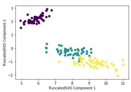

잘 분리 됨, setosa는 특히 잘 분리 됐음

StandardScaler까지 적용하고 SVD와, PCA와 비교해보기

from sklearn.preprocessing import StandardScaler

# iris 데이터를 StandardScaler로 변환
scaler = StandardScaler()
iris_scaled = scaler.fit_transform(iris_ftrs)

# 스케일링된 데이터를 기반으로 TruncatedSVD 변환 수행 
tsvd = TruncatedSVD(n_components=2)
tsvd.fit(iris_scaled)
iris_tsvd = tsvd.transform(iris_scaled)

# 스케일링된 데이터를 기반으로 PCA 변환 수행 
pca = PCA(n_components=2)
pca.fit(iris_scaled)
iris_pca = pca.transform(iris_scaled)

# TruncatedSVD 변환 데이터를 왼쪽에 PCA변환 데이터를 오른쪽에 표현 
fig, (ax1, ax2) = plt.subplots(figsize=(9,4), ncols=2)
ax1.scatter(x=iris_tsvd[:,0], y= iris_tsvd[:,1], c= iris.target)
ax2.scatter(x=iris_pca[:,0], y= iris_pca[:,1], c= iris.target)
ax1.set_title('Truncated SVD Transformed')
ax2.set_title('PCA Transformed')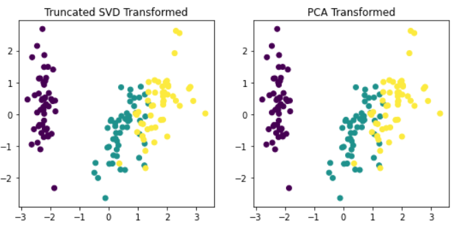

거의 동일함 (같다고 봐도 됨)

---

NMF (참고)

NMF, Non Negative Matrix Factorization, 음수 미포함 행렬 분해

원본 행렬 내의 모든 원소 값이 모두 양수라는 게 보장되면 좀 더 간단하게 두 개의 기반 양수 행렬로 분해될 수 있는 기법

ex) $V_{4\times6} \approx W_{4\times2} \times H_{2\times6}$

행렬 분해: SVD 같은 행렬 분해 기법 통칭
-> 분해된 행렬은 Latent Factor(잠재 요소)를 특성으로 가짐
-> $W$: 원본 행에 대해 이 잠재 요소 값이 얼마나 되는지 대응 (행 크기가 $V$와 같음)
-> $H$: 이 잠재 요소가 원본 열로 어떻게 구성됐는지를 나타냄 (열 크기가 $V$와 같음)

실습

from sklearn.decomposition import NMF
from sklearn.datasets import load_iris
import matplotlib.pyplot as plt
%matplotlib inline

iris = load_iris()
iris_ftrs = iris.data
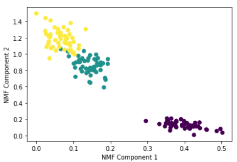
nmf = NMF(n_components=2)

nmf.fit(iris_ftrs)
iris_nmf = nmf.transform(iris_ftrs)

plt.scatter(x=iris_nmf[:,0], y= iris_nmf[:,1], c= iris.target)
plt.xlabel('NMF Component 1')
plt.ylabel('NMF Component 2')