[ML] 군집화 - Gaussian Mixture Model

Gaussian Mixture Model, Mixture of Gaussian, GMM, MoG

Gaussian Mixture Model 개요

거리기반 K-Means의 문제점
-> K-Means는 특정 중심점을 기반으로 거리적으로 퍼져있는 데이터 세트에 군집화를 적용하면 효율적인데 그 반대는 비효율적이다.

예를 들어보자
K-Means는 이런 데이터에서 군집화가 제대로 되지 않는다.
누가봐도 세 개의 군집이 보이는데, 거리 기반의 K-Means는 다음과 같이 군집화한다.

거리 기반으로 이루어지기 때문에 이런 문제가 발생한다.

GMM으로 해보자

예상대로 한 것과 똑같이 군집화가 됐다.

그럼 GMM 군집화는 뭘까?

• 군집화를 적용하고자 하는 데이터가 여러 개의 다른 가우시안 분포를 가지는 모델로 가정하고 군집화를 수행
• 가령 1000개의 데이터 세트가 있다면 이를 구성하는 여러 개의 정규분포 곡선을 추출하고, 개별 데이터가 이 중 어떤 정규분포에 속하는지 결정

GMM은 EM 알고리즘을 사용한다. (사실 K-Means도 이걸 사용함)

EM (Expectation and Maximization)

• Expectation
  -> 개별 데이터 각각에 대해서 특정 정규 분포에 소속될 확률을 구하고 가장 높은 확률을 가진 정규 분포에 소속
  (최초에는 데이터들을 임의로 특정 정규 분포로 소속)
• Maximization
  -> 데이터들이 특정 정규분포로 소속되면 다시 해당 정규분포의 평균과 분산을 구함
  해당 데이터가 발견될 수 있는 가능도를 최대화 (Maximum likelihood) 할 수 있도록 평균과 분산(모수)를 구함

개별 정규분포의 모수인 평균과 분산이 더이상 변경되지 않고
각 개별 데이터들이 이전 정규 분포 소속이 더이상 변경되지 않으면
그것으로 최종 군집화를 결정하고 그렇지 않으면 계속 EM 반복을 수행

-> 이 방법을 수학적으로 설명하면 굉장히 복잡함

---

Gaussian Mixture Model 실습

scikit-learn은 sklearn.mixture.GaussianMixture 클래스 제공

iris 데이터 불러오고 데이터프레임 만들기

from sklearn.datasets import load_iris
from sklearn.cluster import KMeans

import matplotlib.pyplot as plt
import numpy as np
import pandas as pd

iris = load_iris()
feature_names = ['sepal_length','sepal_width','petal_length','petal_width']

irisDF = pd.DataFrame(data=iris.data, columns=feature_names)
irisDF['target'] = iris.target

GMM으로 군집 수 3개로 해서 군집화 진행

from sklearn.mixture import GaussianMixture

gmm = GaussianMixture(n_components=3, random_state=0).fit(iris.data)
gmm_cluster_labels = gmm.predict(iris.data)

# 클러스터링 결과를 irisDF 의 'gmm_cluster' 컬럼명으로 저장
irisDF['gmm_cluster'] = gmm_cluster_labels


# target 값에 따라서 gmm_cluster 값이 어떻게 매핑되었는지 확인. 
iris_result = irisDF.groupby(['target'])['gmm_cluster'].value_counts()
print(iris_result)

target  gmm_cluster
0       0              50
1       2              45
        1               5
2       1              50
Name: gmm_cluster, dtype: int64

K-Means보다 훨씬 잘 된 거 같음
K-Means로 한 것도 다시 봐보자

kmeans = KMeans(n_clusters=3, init='k-means++', max_iter=300,random_state=0).fit(iris.data)
kmeans_cluster_labels = kmeans.predict(iris.data)
irisDF['kmeans_cluster'] = kmeans_cluster_labels
iris_result = irisDF.groupby(['target'])['kmeans_cluster'].value_counts()
print(iris_result)

target  kmeans_cluster
0       1                 50
1       0                 48
        2                  2
2       2                 36
        0                 14
Name: kmeans_cluster, dtype: int64

클러스터링 결과를 시각화하는 함수를 만듦 (뒤에 DBSCAN에서도 사용)
iscenter 인자는 centroid를 표시할지 말지 결정 (GMM은 없음)

### 클러스터 결과를 담은 DataFrame과 사이킷런의 Cluster 객체등을 인자로 받아 클러스터링 결과를 시각화하는 함수  
def visualize_cluster_plot(clusterobj, dataframe, label_name, iscenter=True):
    if iscenter :
        centers = clusterobj.cluster_centers_
        
    unique_labels = np.unique(dataframe[label_name].values)
    markers=['o', 's', '^', 'x', '*']
    isNoise=False

    for label in unique_labels:
        label_cluster = dataframe[dataframe[label_name]==label]
        if label == -1:
            cluster_legend = 'Noise'
            isNoise=True
        else :
            cluster_legend = 'Cluster '+str(label)
        
        plt.scatter(x=label_cluster['ftr1'], y=label_cluster['ftr2'], s=70,\
                    edgecolor='k', marker=markers[label], label=cluster_legend)
        
        if iscenter:
            center_x_y = centers[label]
            plt.scatter(x=center_x_y[0], y=center_x_y[1], s=250, color='white',
                        alpha=0.9, edgecolor='k', marker=markers[label])
            plt.scatter(x=center_x_y[0], y=center_x_y[1], s=70, color='k',\
                        edgecolor='k', marker='$%d$' % label)
    if isNoise:
        legend_loc='upper center'
    else: legend_loc='upper right'
    
    plt.legend(loc=legend_loc)
    plt.show()

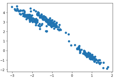
make_blobs로 군집 랜덤 표본을 추출하고
GMM에 적합하게 데이터를 비틀음
-> 앞에 개요에서 봤던 그 데이터임
어떻게 군집 표본 추출 되었는지까지 시각화

from sklearn.datasets import make_blobs

# make_blobs() 로 300개의 데이터 셋, 3개의 cluster 셋, cluster_std=0.5 을 만듬. 
X, y = make_blobs(n_samples=300, n_features=2, centers=3, cluster_std=0.5, random_state=0)

# 길게 늘어난 타원형의 데이터 셋을 생성하기 위해 변환함. 
transformation = [[0.60834549, -0.63667341], [-0.40887718, 0.85253229]]
X_aniso = np.dot(X, transformation)
# feature 데이터 셋과 make_blobs( ) 의 y 결과 값을 DataFrame으로 저장
clusterDF = pd.DataFrame(data=X_aniso, columns=['ftr1', 'ftr2'])
clusterDF['target'] = y
# 생성된 데이터 셋을 target 별로 다른 marker 로 표시하여 시각화 함. 
visualize_cluster_plot(None, clusterDF, 'target', iscenter=False)

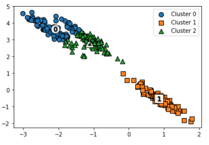
K-Means 군집화 진행 후 시각화하기

# 3개의 Cluster 기반 Kmeans 를 X_aniso 데이터 셋에 적용 
kmeans = KMeans(3, random_state=0)
kmeans_label = kmeans.fit_predict(X_aniso)
clusterDF['kmeans_label'] = kmeans_label

visualize_cluster_plot(kmeans, clusterDF, 'kmeans_label',iscenter=True)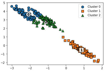

거리 기반 특성상 이렇게 군집화가 되어버림

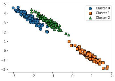
GMM 군집화 진행 후 시각화하기

# 3개의 n_components기반 GMM을 X_aniso 데이터 셋에 적용 
gmm = GaussianMixture(n_components=3, random_state=0)
gmm_label = gmm.fit(X_aniso).predict(X_aniso)
clusterDF['gmm_label'] = gmm_label

# GaussianMixture는 cluster_centers_ 속성이 없으므로 iscenter를 False로 설정. 
visualize_cluster_plot(gmm, clusterDF, 'gmm_label',iscenter=False)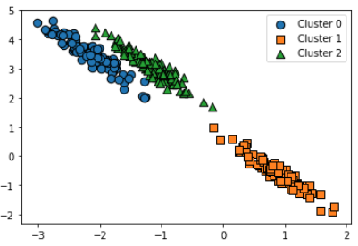

의도한 것과 동일하게 됐음!

둘을 비교해보자

print('### KMeans Clustering ###')
print(clusterDF.groupby('target')['kmeans_label'].value_counts())
print('\n### Gaussian Mixture Clustering ###')
print(clusterDF.groupby('target')['gmm_label'].value_counts())

### KMeans Clustering ###
target  kmeans_label
0       2                73
        0                27
1       1               100
2       0                86
        2                14
Name: kmeans_label, dtype: int64

### Gaussian Mixture Clustering ###
target  gmm_label
0       2            100
1       1            100
2       0            100
Name: gmm_label, dtype: int64

GMM은 의도와 100% 일치하게 군집화 됨!