새싹 인공지능 응용sw 개발자 양성 교육 프로그램 심선조 강사님 수업 정리 글입니다.
모델 쓰는 방법은 비슷하지만
데이터 전처리를 어떻게 하느냐에 따라 달라진다.
기본 공통 상황은 1. null값처리 2.글자->숫자 3.분류면 이진분류에 따라 처리, 회귀면 숫자 크기에 영향을 받기때문에 정규화, 레이블인코딩을 통해 숫자값을 줄여준다. target이 정규분포 형태인지 확인, 이상치 확인, 회귀 모델은 숫자값에 크기, 상관계수에 영향을 받는다.
- 교재 375p
회귀 실습 - 캐글 주택 가격: 고급 회귀 기법
https://www.kaggle.com/competitions/house-prices-advanced-regression-techniques
import pandas as pd
import numpy as np
import seaborn as sns
import matplotlib.pyplot as plt
import warnings
warnings.filterwarnings('ignore')
df = pd.read_csv('houseprice.csv')df.head(2)| Id | MSSubClass | MSZoning | LotFrontage | LotArea | Street | Alley | LotShape | LandContour | Utilities | ... | PoolArea | PoolQC | Fence | MiscFeature | MiscVal | MoSold | YrSold | SaleType | SaleCondition | SalePrice | |
|---|---|---|---|---|---|---|---|---|---|---|---|---|---|---|---|---|---|---|---|---|---|
| 0 | 1 | 60 | RL | 65.0 | 8450 | Pave | NaN | Reg | Lvl | AllPub | ... | 0 | NaN | NaN | NaN | 0 | 2 | 2008 | WD | Normal | 208500 |
| 1 | 2 | 20 | RL | 80.0 | 9600 | Pave | NaN | Reg | Lvl | AllPub | ... | 0 | NaN | NaN | NaN | 0 | 5 | 2007 | WD | Normal | 181500 |
2 rows × 81 columns
df.info()<class 'pandas.core.frame.DataFrame'>
RangeIndex: 1460 entries, 0 to 1459
Data columns (total 81 columns):
# Column Non-Null Count Dtype
--- ------ -------------- -----
0 Id 1460 non-null int64
1 MSSubClass 1460 non-null int64
2 MSZoning 1460 non-null object
3 LotFrontage 1201 non-null float64
4 LotArea 1460 non-null int64
5 Street 1460 non-null object
6 Alley 91 non-null object
7 LotShape 1460 non-null object
8 LandContour 1460 non-null object
9 Utilities 1460 non-null object
10 LotConfig 1460 non-null object
11 LandSlope 1460 non-null object
12 Neighborhood 1460 non-null object
13 Condition1 1460 non-null object
14 Condition2 1460 non-null object
15 BldgType 1460 non-null object
16 HouseStyle 1460 non-null object
17 OverallQual 1460 non-null int64
18 OverallCond 1460 non-null int64
19 YearBuilt 1460 non-null int64
20 YearRemodAdd 1460 non-null int64
21 RoofStyle 1460 non-null object
22 RoofMatl 1460 non-null object
23 Exterior1st 1460 non-null object
24 Exterior2nd 1460 non-null object
25 MasVnrType 1452 non-null object
26 MasVnrArea 1452 non-null float64
27 ExterQual 1460 non-null object
28 ExterCond 1460 non-null object
29 Foundation 1460 non-null object
30 BsmtQual 1423 non-null object
31 BsmtCond 1423 non-null object
32 BsmtExposure 1422 non-null object
33 BsmtFinType1 1423 non-null object
34 BsmtFinSF1 1460 non-null int64
35 BsmtFinType2 1422 non-null object
36 BsmtFinSF2 1460 non-null int64
37 BsmtUnfSF 1460 non-null int64
38 TotalBsmtSF 1460 non-null int64
39 Heating 1460 non-null object
40 HeatingQC 1460 non-null object
41 CentralAir 1460 non-null object
42 Electrical 1459 non-null object
43 1stFlrSF 1460 non-null int64
44 2ndFlrSF 1460 non-null int64
45 LowQualFinSF 1460 non-null int64
46 GrLivArea 1460 non-null int64
47 BsmtFullBath 1460 non-null int64
48 BsmtHalfBath 1460 non-null int64
49 FullBath 1460 non-null int64
50 HalfBath 1460 non-null int64
51 BedroomAbvGr 1460 non-null int64
52 KitchenAbvGr 1460 non-null int64
53 KitchenQual 1460 non-null object
54 TotRmsAbvGrd 1460 non-null int64
55 Functional 1460 non-null object
56 Fireplaces 1460 non-null int64
57 FireplaceQu 770 non-null object
58 GarageType 1379 non-null object
59 GarageYrBlt 1379 non-null float64
60 GarageFinish 1379 non-null object
61 GarageCars 1460 non-null int64
62 GarageArea 1460 non-null int64
63 GarageQual 1379 non-null object
64 GarageCond 1379 non-null object
65 PavedDrive 1460 non-null object
66 WoodDeckSF 1460 non-null int64
67 OpenPorchSF 1460 non-null int64
68 EnclosedPorch 1460 non-null int64
69 3SsnPorch 1460 non-null int64
70 ScreenPorch 1460 non-null int64
71 PoolArea 1460 non-null int64
72 PoolQC 7 non-null object
73 Fence 281 non-null object
74 MiscFeature 54 non-null object
75 MiscVal 1460 non-null int64
76 MoSold 1460 non-null int64
77 YrSold 1460 non-null int64
78 SaleType 1460 non-null object
79 SaleCondition 1460 non-null object
80 SalePrice 1460 non-null int64
dtypes: float64(3), int64(35), object(43)
memory usage: 924.0+ KBisnull_series = df.isnull().sum()isnull_series[isnull_series>0].sort_values(ascending=False) #0인거 빼고 확인 가능PoolQC 1453
MiscFeature 1406
Alley 1369
Fence 1179
FireplaceQu 690
LotFrontage 259
GarageType 81
GarageYrBlt 81
GarageFinish 81
GarageQual 81
GarageCond 81
BsmtExposure 38
BsmtFinType2 38
BsmtFinType1 37
BsmtCond 37
BsmtQual 37
MasVnrArea 8
MasVnrType 8
Electrical 1
dtype: int64#회귀에서 target이 정규분포 형태이면 성능이 좋아진다.
plt.xticks(rotation=45)
sns.histplot(df['SalePrice'],kde=True) #히스토그램은 연속된 데이터를 구간을 나누어서 해당 구간안에 데이터가 들어가는 갯수를 세어 표시해 준다.
#df['SalePrice'] = target값, 종속변수
plt.show()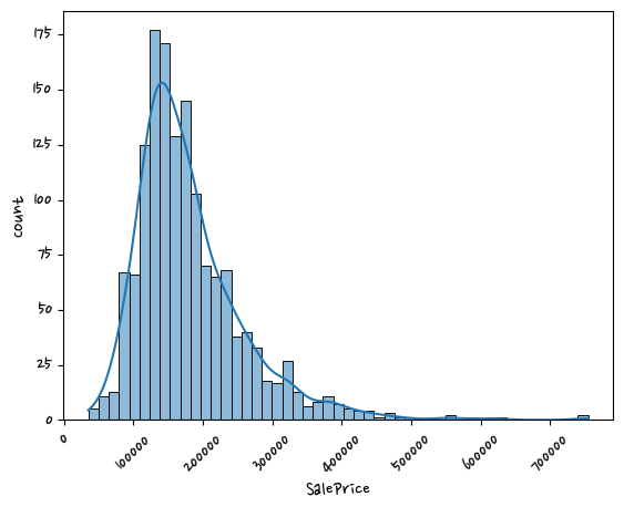
log 쓰면 좋은 점 expm1 -1취한다. 원래 값으로 돌리는 것도 가능하다.
log_saleprice = np.log1p(df['SalePrice'])
sns.histplot(log_saleprice,kde=True)
<AxesSubplot:xlabel='SalePrice', ylabel='Count'>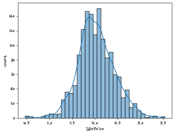
나머지 null 피처는 null값이 많지 않으므로 숫자형의 경우 평균값으로 대체
original_saleprice = df['SalePrice']
df['SalePrice'] = np.log1p(df['SalePrice'])
df.drop(columns=['PoolQC', 'MiscFeature', 'Alley', 'Fence', 'FireplaceQu', 'Id'],inplace=True)
df.fillna(df.mean(),inplace=True)
null_column_count = df.isnull().sum()[df.isnull().sum()>0] #object는 null값이 그대로 남아 있다. fillna를 통해 mean값으로 채웠다. mean값으로 채워진 값들은 숫자형이다. object타입의 null은 그대로 남아 있다.df.dtypes[null_column_count.index]#null_column_count가 series라서 index(=컬럼이름)가 있다.MasVnrType object
BsmtQual object
BsmtCond object
BsmtExposure object
BsmtFinType1 object
BsmtFinType2 object
Electrical object
GarageType object
GarageFinish object
GarageQual object
GarageCond object
dtype: object문자형 피처를 제외하고 null값이 없다. 문자열은 원핫인코딩을 할 것이다.
원핫인코딩은 판다스의 get_dummies()로 이용 (null값에 대한 처리도 값이 처리됨, null값 -> 0으로 변환)
df.shape #데이터 건수 확인(1460, 75)df_ohe = pd.get_dummies(df) #ohe = 원핫인코딩df_ohe.shape #데이터 건수는 그대로, 컬럼은 증가, 하나의 컬럼에 유일값을 뽑은 만큼 컬럼이 늘어난다.(1460, 271)선형 회귀 모델 학습/예측/평가
R이 붙는다 root씌운 것
예측 평가는 RMSLE(실제값과 예측값의 오류를 로그 변환한 뒤 RMSE를 적용)
이미 타깃 값에는 로그 처리 됨
def get_rmse(model):
    from sklearn.metrics import mean_squared_error
    import numpy as np
    pred = model.predict(X_test)
    mse = mean_squared_error(y_test, pred)
    rmse = np.sqrt(mse) #sqrt = 스퀘어 루트, 루트 씌어줌
    print(model.__class__.__name__,'로그 변환된 RMSE:', np.round(rmse,3))# class 이름을 print해줌
    return rmse

def get_rmses(models): #모델은 linear, ridge, lasso등등 있는 데 알아서 모델들 안에 넣어 준다.
    rmses=[]
    for model in models:
        rmse = get_rmse(model)
        rmses.append(rmse)
    return rmses
from sklearn.linear_model import LinearRegression,Ridge,Lasso #LinearRegression = 일반 선형회귀, Ridge(l2규제),Lasso(l1규제) = 규제
from sklearn.model_selection import train_test_split(l1규제) : 회귀계수를 줄여서 0이 되도록 , (l2규제) : 줄이지만 0이 되진 않는다. , 엘라스틱규제 : l1보다는 적게 없어지게 조절한다. 0이되면 feature가 사라진다.
회귀 계수 = w, 변수마다 하나씩 있다. 회귀 계수는 점점 커지는 경향이 있다. 너무 커지면 가적합문제가 발생한다. 실제 데이터가 들어오면 예측결과가 떨어지는 문제가 발생할 수도 있다.
y = df_ohe['SalePrice']
X = df_ohe.drop(columns=['SalePrice'])X_train,X_test,y_train,y_test = train_test_split(X,y,test_size=0.2,random_state=156)lr_reg = LinearRegression()
lr_reg.fit(X_train,y_train)
ridge_reg = Ridge()
ridge_reg.fit(X_train,y_train)
lasso_reg = Lasso()
lasso_reg.fit(X_train,y_train)
#학습끝
models=[lr_reg, ridge_reg,lasso_reg] #리스트 만듦
get_rmses(models)LinearRegression 로그 변환된 RMSE: 0.132
Ridge 로그 변환된 RMSE: 0.128
Lasso 로그 변환된 RMSE: 0.176
[0.13189576579154494, 0.12750846334052998, 0.17628250556471403]np.expm1(0.13189576579154494) #원래값으로 리턴됨0.14098938294353924- 교재 382p
def get_top_bottom_coef(model, n=10):
    coef = pd.Series(model.coef_,index=X.columns)
    coef_high = coef.sort_values(ascending=False).head(n)
    coef_low = coef.sort_values(ascending=False).tail(n)
return coef_high,coef_lowget_top_bottom_coef(lr_reg) #모델을 넣어주면 회귀계수값이 나옴(RoofMatl_Membran 0.528057
RoofMatl_Metal 0.414453
RoofMatl_WdShngl 0.345254
RoofMatl_Roll 0.311983
RoofStyle_Shed 0.292647
RoofMatl_CompShg 0.273884
GarageQual_Ex 0.261599
Condition2_RRNn 0.260054
RoofMatl_WdShake 0.256344
RoofMatl_Tar&Grv 0.242292
dtype: float64,
Neighborhood_MeadowV -0.228006
Condition2_RRAe -0.243308
Electrical_FuseP -0.258129
Heating_Grav -0.264520
GarageCond_Ex -0.265441
Electrical_Mix -0.300984
MSZoning_C (all) -0.323040
Functional_Maj2 -0.426389
Condition2_PosN -0.663744
RoofMatl_ClyTile -2.372268
dtype: float64)get_top_bottom_coef(lr_reg,3)(RoofMatl_Membran 0.528057
RoofMatl_Metal 0.414453
RoofMatl_WdShngl 0.345254
dtype: float64,
Functional_Maj2 -0.426389
Condition2_PosN -0.663744
RoofMatl_ClyTile -2.372268
dtype: float64)#회귀계수를 시각화
def visualize_coefficient(models):
fig,axs = plt.subplots(figsize=(24, 10), nrows=1, ncols=3)
fig.tight_layout() #tight_layout() = 배치를 맞춰줌
for i_num, model in enumerate(models): #i_num, model = index
coef_high,coef_low = get_top_bottom_coef(model)
coef_concat = pd.concat([coef_high,coef_low])
axs[i_num].set_title(model.__class__.__name__+'Coefficient',size=25)
axs[i_num].tick_params(axis='y', direction='in', pad=-120) #direction='in' 글자가 그래프 안에 들어와도 된다
for lable in (axs[i_num].get_xticklabels()+axs[i_num].get_yticklabels()):
lable.set_fontsize(22)
sns.barplot(x=coef_concat.values,y=coef_concat.index, ax=axs[i_num]) #series라서 .values 사용visualize_coefficient(models)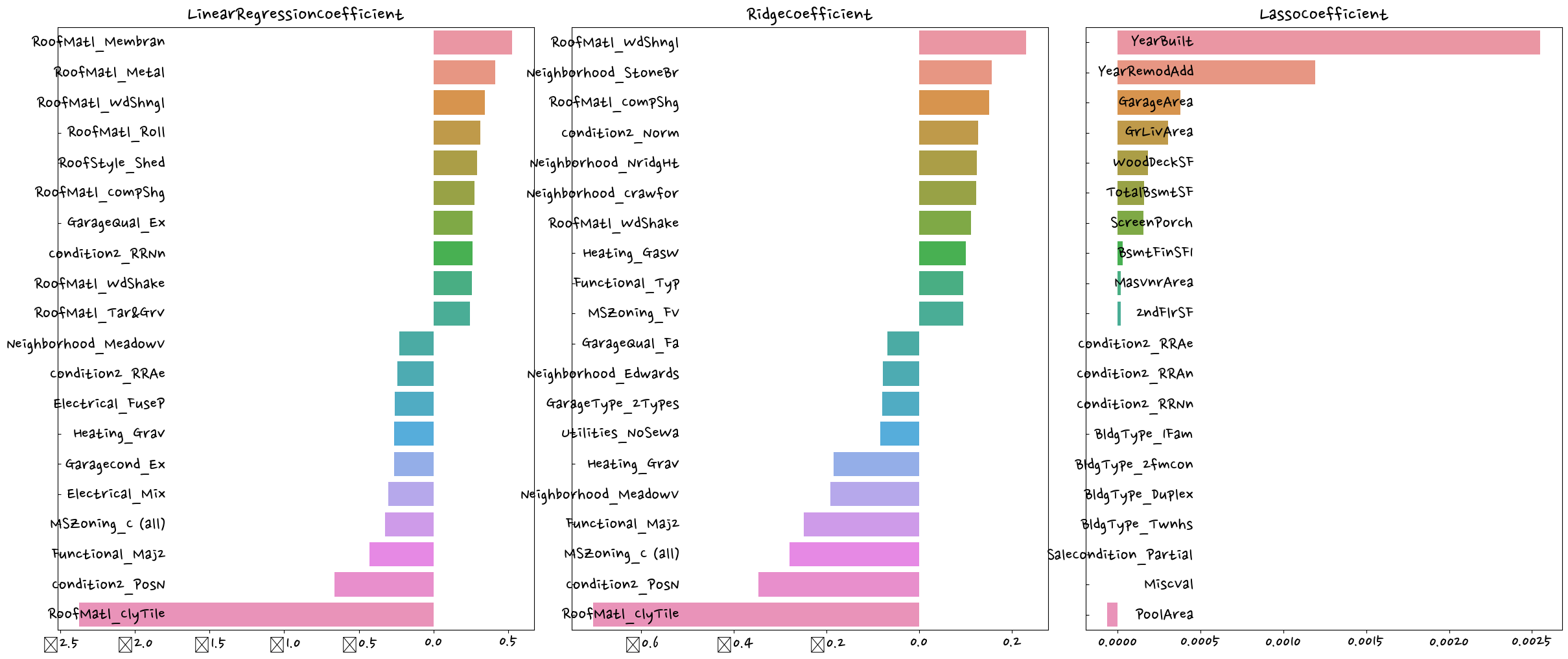
라쏘의 경우 다른 두 개의 모델과 다른 회귀 계수 형태를 보이고 있다. -> 교차 검증
target은 정규분포로 바꿈.
이상치가 있으면 성능이 떨어져서 이상치 여부 확인해서 이상치 처리.
기본적인 처리가 끝나면
from sklearn.model_selection import cross_val_scoredef get_avg_rmse_cv(models):
for model in models:
rmse_list = np.sqrt(-cross_val_score(model,X,y,scoring='neg_mean_squared_error',cv=5)) #rmse = 5개가 나올 것
rmse_avg = np.mean(rmse_list)
print(f'{model.__class__.__name__} cv rmse 값 리스트 : {np.round(rmse_list,3)}')
print(f'{model.__class__.__name__} cv 평균 rmse 값 : {np.round(rmse_avg,3)}')get_avg_rmse_cv(models)LinearRegression cv rmse 값 리스트 : [0.135 0.165 0.168 0.111 0.198]
LinearRegression cv 평균 rmse 값 : 0.155
Ridge cv rmse 값 리스트 : [0.117 0.154 0.142 0.117 0.189]
Ridge cv 평균 rmse 값 : 0.144
Lasso cv rmse 값 리스트 : [0.161 0.204 0.177 0.181 0.265]
Lasso cv 평균 rmse 값 : 0.198from sklearn.model_selection import GridSearchCVdef print_best_params(model,params):
grid_model = GridSearchCV(model,params,scoring='neg_mean_squared_error', cv=5) #GridSearchCV라서 scoring='neg' #scoring='neg_mean_squared_error' 예측값과 차이의 제곱?
grid_model.fit(X,y)
rmse = np.sqrt(-1*grid_model.best_score_)
print(f'{model.__class__.__name__} 5 cv시 최적 평균 rmse 값:{np.round(rmse, 4)}, 최적 alpha값:{grid_model.best_params_}')ridge_param = {
'alpha':[0.05, 0.1, 1, 5, 8, 10, 12, 15, 20]
} #ridge더 크게 rasso 더 작게
print_best_params(ridge_reg, ridge_param)Ridge 5 cv시 최적 평균 rmse 값:0.1418, 최적 alpha값:{'alpha': 12}lasso_param = {'alpha':[0.001, 0.005, 0.008, 0.05, 0.05, 0.1, 0.5, 1, 5, 10]}
print_best_params(lasso_reg, lasso_param)Lasso 5 cv시 최적 평균 rmse 값:0.142, 최적 alpha값:{'alpha': 0.001}최적 ridge = 0.1 , rasso =0.1
lr_reg = LinearRegression()
lr_reg.fit(X_train,y_train)

ridge_reg = Ridge(alpha=12)
ridge_reg.fit(X_train,y_train)

lasso_reg = Lasso(alpha=0.001)
lasso_reg.fit(X_train,y_train)

models=[lr_reg, ridge_reg,lasso_reg]
get_rmses(models)

visualize_coefficient(models)
LinearRegression 로그 변환된 RMSE: 0.132
Ridge 로그 변환된 RMSE: 0.124
Lasso 로그 변환된 RMSE: 0.12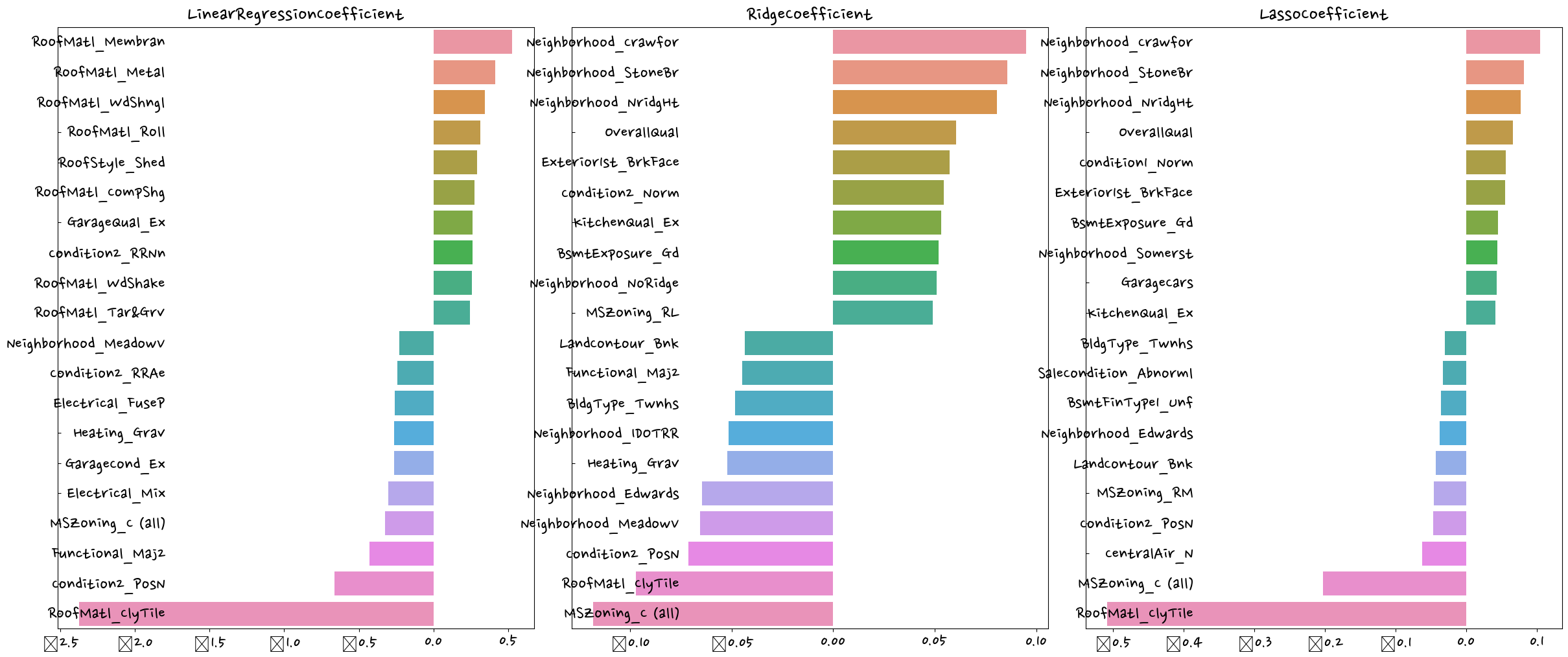
파라미터 튜닝을 통해 ~~비슷한 양상을 보인다?
회귀는 (정규)분포가 중요하다.
- from scipy.stats import skew : 왜곡정도 확인
일반적으로 skew()함수의 반환 값이 1 이상인 경우를 왜곡 정도가 높다고 판단하지만 상황에 따라 편차가 있다.
from scipy.stats import skew#object가 아닌 숫자형 피처의 컬럼 index객체 추출
feature_index = df.dtypes[df.dtypes != 'object'].index#df에 칼럼 index를 []로 입력하면 해당하는 칼럼 데이터 세트 반환. apply lambda로 skew() 호출
skew_features = df[feature_index].apply(lambda x:skew(x))#skew(왜곡) 정도가 1이상인 칼럼만 추출
skew_features_top = skew_features[skew_features>1]skew_features_top.sort_values(ascending=False)MiscVal 24.451640
PoolArea 14.813135
LotArea 12.195142
3SsnPorch 10.293752
LowQualFinSF 9.002080
KitchenAbvGr 4.483784
BsmtFinSF2 4.250888
ScreenPorch 4.117977
BsmtHalfBath 4.099186
EnclosedPorch 3.086696
MasVnrArea 2.673661
LotFrontage 2.382499
OpenPorchSF 2.361912
BsmtFinSF1 1.683771
WoodDeckSF 1.539792
TotalBsmtSF 1.522688
MSSubClass 1.406210
1stFlrSF 1.375342
GrLivArea 1.365156
dtype: float64df[skew_features_top.index] = np.log1p(df[skew_features_top.index])df_ohe = pd.get_dummies(df)
y = df_ohe['SalePrice']
X = df_ohe.drop(columns=['SalePrice'])
X_train,X_test,y_train,y_test = train_test_split(X,y,test_size=0.2,random_state=156)
ridge_param = {'alpha':[0.05, 0.1, 1, 5, 8, 10, 12, 15, 20]}
print_best_params(ridge_reg, ridge_param)
alsso_param = {'alpha':[0.001, 0.005, 0.008, 0.05, 0.05, 0.1, 0.5, 1, 5, 10]}
print_best_params(lasso_reg, lasso_param)Ridge 5 cv시 최적 평균 rmse 값:0.1275, 최적 alpha값:{'alpha': 10}
Lasso 5 cv시 최적 평균 rmse 값:0.1252, 최적 alpha값:{'alpha': 0.001}lr_reg = LinearRegression()
lr_reg.fit(X_train,y_train)
ridge_reg = Ridge(alpha=12)
ridge_reg.fit(X_train,y_train)
lasso_reg = Lasso(alpha=0.001)
lasso_reg.fit(X_train,y_train)
models=[lr_reg, ridge_reg,lasso_reg]
get_rmses(models)
visualize_coefficient(models)LinearRegression 로그 변환된 RMSE: 0.128
Ridge 로그 변환된 RMSE: 0.122
Lasso 로그 변환된 RMSE: 0.119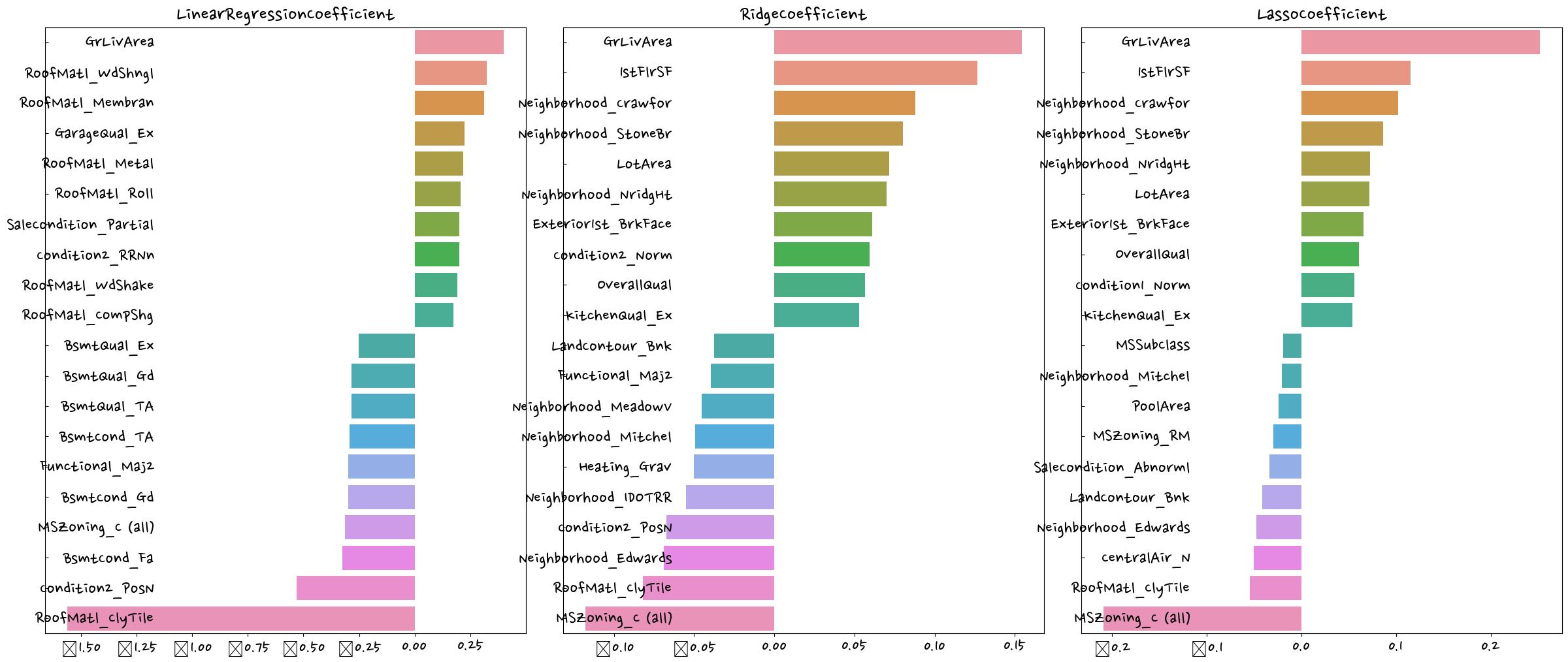
- 이상치 확인
종속변수에 영향을 주는 독립변수
상관계수가 높은 쪽으로 이상치를 처리하는 것이 효과적이다.
회귀계수가 크다 (= 결과값에 영향을 많이 미친다)
df_org = pd.read_csv('houseprice.csv')
plt.scatter(x=df_org['GrLivArea'],y=df_org['SalePrice']) #df_org(original) #'GrLivArea': 지상 거실 면적<matplotlib.collections.PathCollection at 0x2c134dc3400>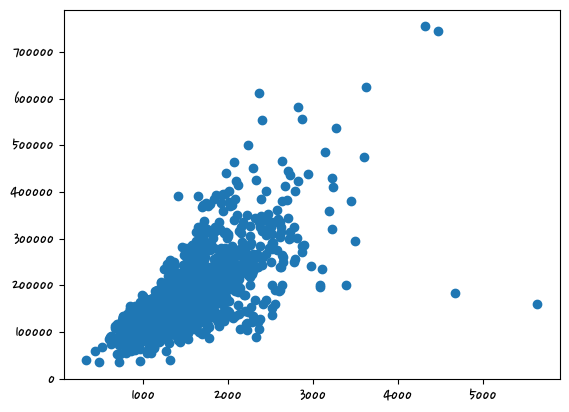
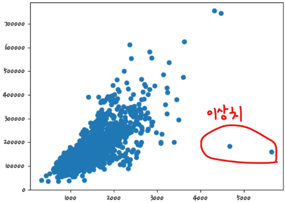
cond1 = df_ohe['GrLivArea'] > np.log1p(4000) #원핫인코딩까지 되어 있다, 가격에 로그처리됨 #cond1 = 조건
#로그처리해서 조건을 줘야 한다. -> np.log1p(4000)
cond2 = df_ohe['SalePrice'] < np.log1p(500000)
outlier_index = df_ohe[cond1 & cond2].indexdf_ohe.shape(1458, 271)df_ohe.drop(index=outlier_index,inplace=True)df_ohe.shape #이상치(2건) 제거됨(1458, 271)y = df_ohe['SalePrice']
X = df_ohe.drop(columns=['SalePrice'])
X_train,X_test,y_train,y_test = train_test_split(X,y,test_size=0.2,random_state=156)
ridge_param = {'alpha':[0.05, 0.1, 1, 5, 8, 10, 12, 15, 20]}
print_best_params(ridge_reg, ridge_param)
alsso_param = {'alpha':[0.001, 0.005, 0.008, 0.05, 0.05, 0.1, 0.5, 1, 5, 10]}
print_best_params(lasso_reg, lasso_param)Ridge 5 cv시 최적 평균 rmse 값:0.1125, 최적 alpha값:{'alpha': 8}
Lasso 5 cv시 최적 평균 rmse 값:0.1122, 최적 alpha값:{'alpha': 0.001}lr_reg = LinearRegression()
lr_reg.fit(X_train,y_train)
ridge_reg = Ridge(alpha=12)
ridge_reg.fit(X_train,y_train)
lasso_reg = Lasso(alpha=0.001)
lasso_reg.fit(X_train,y_train)
models=[lr_reg, ridge_reg,lasso_reg]
get_rmses(models)
visualize_coefficient(models)
# LinearRegression 로그 변환된 RMSE: 0.128
# Ridge 로그 변환된 RMSE: 0.122
# Lasso 로그 변환된 RMSE: 0.119LinearRegression 로그 변환된 RMSE: 0.129
Ridge 로그 변환된 RMSE: 0.103
Lasso 로그 변환된 RMSE: 0.1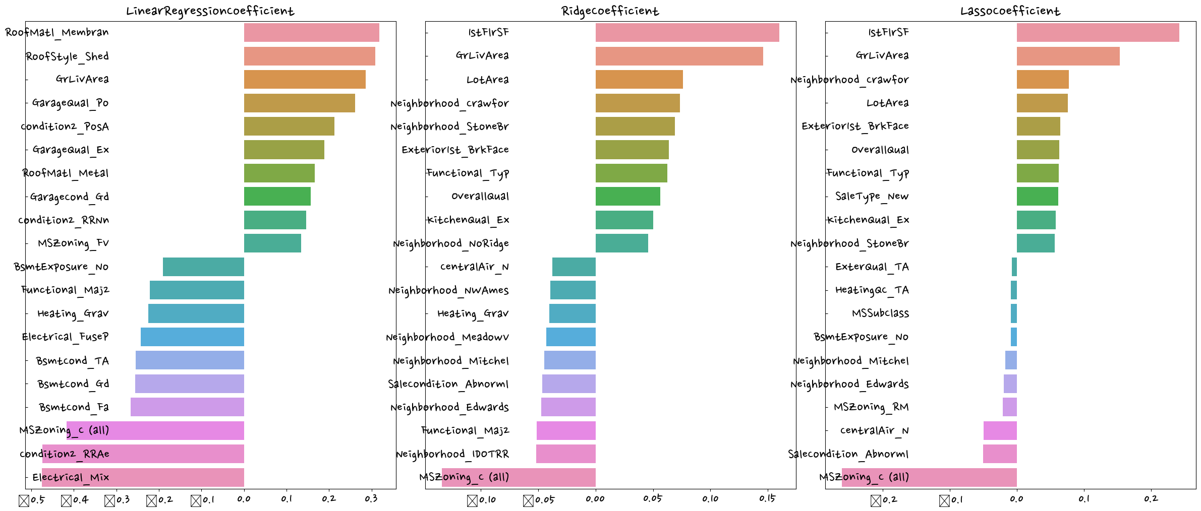
회귀 트리 모델 학습/예측/평가
- 교재 391p
lightbgm, xgboost - 회귀, 분류둘 다 있다
정리
선형 회귀는 뎅터 값의 분포도와 인코딩 방법에 많은 영향을 받을 수 있다.
선형 회귀는 데이터 값의 분포도가 정규분포와 같은 종 모양의 형태를 선호
타깃값의 분포도가 왜곡(skew)되지 않고 정규 분포 형태로 되어야 에측 성능을 저하시키지 않는다.
차원축소
- 교재 399p
차원 = 변수
차원이 증가할수록 데이터 포인트 간의 거리가 기하급수적으로 멀어지게 되고, 희소(sparse)한 구조를 가지게 된다.
피처간의 상관관계까 높을 경우 다중 공선성 문제로 모델의 예측 서능이 저하된다.
PCA
차원을 여러개 합쳐서 사용하는 것이다. 데이터 변동성이 가장 큰 방향으로 축을 생성하고, 새롭게 생성된 축으로 데이터를 투영하는 방식
PCA는 제일 먼저 가장 큰 데이터 변동성(Variance)을 기반으로 첫 번째 벡터 축을 생성하고, 두번 째 축은 이 벡터 축에 직각이 되는 벡터(직교 벡터)를 축으로 한다.
세 번째 축은 다시 두 번째 축과 직각이 되는 벡터를 설정하는 방식으로 축을 생성한다.
from sklearn.datasets import load_iris
import pandas as pd
import matplotlib.pyplot as plt
iris = load_iris(as_frame=True)iris.data.columns = ['sepal length', 'sepal width', 'petal length','petal width']iris.data| sepal length | sepal width | petal length | petal width | |
|---|---|---|---|---|
| 0 | 5.1 | 3.5 | 1.4 | 0.2 |
| 1 | 4.9 | 3.0 | 1.4 | 0.2 |
| 2 | 4.7 | 3.2 | 1.3 | 0.2 |
| 3 | 4.6 | 3.1 | 1.5 | 0.2 |
| 4 | 5.0 | 3.6 | 1.4 | 0.2 |
| ... | ... | ... | ... | ... |
| 145 | 6.7 | 3.0 | 5.2 | 2.3 |
| 146 | 6.3 | 2.5 | 5.0 | 1.9 |
| 147 | 6.5 | 3.0 | 5.2 | 2.0 |
| 148 | 6.2 | 3.4 | 5.4 | 2.3 |
| 149 | 5.9 | 3.0 | 5.1 | 1.8 |
150 rows × 4 columns
iris.target #series형태0 0
1 0
2 0
3 0
4 0
..
145 2
146 2
147 2
148 2
149 2
Name: target, Length: 150, dtype: int32iris.data['target'] = iris.target
iris.data.head(2)| sepal length | sepal width | petal length | petal width | target | |
|---|---|---|---|---|---|
| 0 | 5.1 | 3.5 | 1.4 | 0.2 | 0 |
| 1 | 4.9 | 3.0 | 1.4 | 0.2 | 0 |
df = iris.data markers=['^','s','o']
for i, marker in enumerate(markers):
x = df[df['target']==i]['sepal length']
y = df[df['target']==i]['sepal width']
plt.scatter(x,y,marker=marker,label=iris.target_names[i])
plt.legend()
plt.show()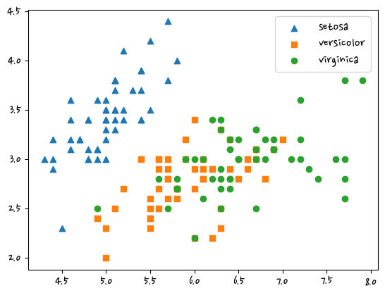
pca적용하기 전에 개별 속성을 함께 스케일링해야 한다. standascale은 평균 0, 분산 1로 만들어준다.
from sklearn.preprocessing import StandardScalerdf_scaled = StandardScaler().fit_transform(df.iloc[:,:-1]) #df.iloc[:,:-1] 행은 전부다, 열은 뒤에 거 빼고
df_scaledarray([[-9.00681170e-01, 1.01900435e+00, -1.34022653e+00,
-1.31544430e+00],
[-1.14301691e+00, -1.31979479e-01, -1.34022653e+00,
-1.31544430e+00],
[-1.38535265e+00, 3.28414053e-01, -1.39706395e+00,
-1.31544430e+00],
[-1.50652052e+00, 9.82172869e-02, -1.28338910e+00,
-1.31544430e+00],
[-1.02184904e+00, 1.24920112e+00, -1.34022653e+00,
-1.31544430e+00],
[-5.37177559e-01, 1.93979142e+00, -1.16971425e+00,
-1.05217993e+00],
[-1.50652052e+00, 7.88807586e-01, -1.34022653e+00,
-1.18381211e+00],
[-1.02184904e+00, 7.88807586e-01, -1.28338910e+00,
-1.31544430e+00],
[-1.74885626e+00, -3.62176246e-01, -1.34022653e+00,
-1.31544430e+00],
[-1.14301691e+00, 9.82172869e-02, -1.28338910e+00,
-1.44707648e+00],
[-5.37177559e-01, 1.47939788e+00, -1.28338910e+00,
-1.31544430e+00],
[-1.26418478e+00, 7.88807586e-01, -1.22655167e+00,
-1.31544430e+00],
[-1.26418478e+00, -1.31979479e-01, -1.34022653e+00,
-1.44707648e+00],
[-1.87002413e+00, -1.31979479e-01, -1.51073881e+00,
-1.44707648e+00],
[-5.25060772e-02, 2.16998818e+00, -1.45390138e+00,
-1.31544430e+00],
[-1.73673948e-01, 3.09077525e+00, -1.28338910e+00,
-1.05217993e+00],
[-5.37177559e-01, 1.93979142e+00, -1.39706395e+00,
-1.05217993e+00],
[-9.00681170e-01, 1.01900435e+00, -1.34022653e+00,
-1.18381211e+00],
[-1.73673948e-01, 1.70959465e+00, -1.16971425e+00,
-1.18381211e+00],
[-9.00681170e-01, 1.70959465e+00, -1.28338910e+00,
-1.18381211e+00],
[-5.37177559e-01, 7.88807586e-01, -1.16971425e+00,
-1.31544430e+00],
[-9.00681170e-01, 1.47939788e+00, -1.28338910e+00,
-1.05217993e+00],
[-1.50652052e+00, 1.24920112e+00, -1.56757623e+00,
-1.31544430e+00],
[-9.00681170e-01, 5.58610819e-01, -1.16971425e+00,
-9.20547742e-01],
[-1.26418478e+00, 7.88807586e-01, -1.05603939e+00,
-1.31544430e+00],
[-1.02184904e+00, -1.31979479e-01, -1.22655167e+00,
-1.31544430e+00],
[-1.02184904e+00, 7.88807586e-01, -1.22655167e+00,
-1.05217993e+00],
[-7.79513300e-01, 1.01900435e+00, -1.28338910e+00,
-1.31544430e+00],
[-7.79513300e-01, 7.88807586e-01, -1.34022653e+00,
-1.31544430e+00],
[-1.38535265e+00, 3.28414053e-01, -1.22655167e+00,
-1.31544430e+00],
[-1.26418478e+00, 9.82172869e-02, -1.22655167e+00,
-1.31544430e+00],
[-5.37177559e-01, 7.88807586e-01, -1.28338910e+00,
-1.05217993e+00],
[-7.79513300e-01, 2.40018495e+00, -1.28338910e+00,
-1.44707648e+00],
[-4.16009689e-01, 2.63038172e+00, -1.34022653e+00,
-1.31544430e+00],
[-1.14301691e+00, 9.82172869e-02, -1.28338910e+00,
-1.31544430e+00],
[-1.02184904e+00, 3.28414053e-01, -1.45390138e+00,
-1.31544430e+00],
[-4.16009689e-01, 1.01900435e+00, -1.39706395e+00,
-1.31544430e+00],
[-1.14301691e+00, 1.24920112e+00, -1.34022653e+00,
-1.44707648e+00],
[-1.74885626e+00, -1.31979479e-01, -1.39706395e+00,
-1.31544430e+00],
[-9.00681170e-01, 7.88807586e-01, -1.28338910e+00,
-1.31544430e+00],
[-1.02184904e+00, 1.01900435e+00, -1.39706395e+00,
-1.18381211e+00],
[-1.62768839e+00, -1.74335684e+00, -1.39706395e+00,
-1.18381211e+00],
[-1.74885626e+00, 3.28414053e-01, -1.39706395e+00,
-1.31544430e+00],
[-1.02184904e+00, 1.01900435e+00, -1.22655167e+00,
-7.88915558e-01],
[-9.00681170e-01, 1.70959465e+00, -1.05603939e+00,
-1.05217993e+00],
[-1.26418478e+00, -1.31979479e-01, -1.34022653e+00,
-1.18381211e+00],
[-9.00681170e-01, 1.70959465e+00, -1.22655167e+00,
-1.31544430e+00],
[-1.50652052e+00, 3.28414053e-01, -1.34022653e+00,
-1.31544430e+00],
[-6.58345429e-01, 1.47939788e+00, -1.28338910e+00,
-1.31544430e+00],
[-1.02184904e+00, 5.58610819e-01, -1.34022653e+00,
-1.31544430e+00],
[ 1.40150837e+00, 3.28414053e-01, 5.35408562e-01,
2.64141916e-01],
[ 6.74501145e-01, 3.28414053e-01, 4.21733708e-01,
3.95774101e-01],
[ 1.28034050e+00, 9.82172869e-02, 6.49083415e-01,
3.95774101e-01],
[-4.16009689e-01, -1.74335684e+00, 1.37546573e-01,
1.32509732e-01],
[ 7.95669016e-01, -5.92373012e-01, 4.78571135e-01,
3.95774101e-01],
[-1.73673948e-01, -5.92373012e-01, 4.21733708e-01,
1.32509732e-01],
[ 5.53333275e-01, 5.58610819e-01, 5.35408562e-01,
5.27406285e-01],
[-1.14301691e+00, -1.51316008e+00, -2.60315415e-01,
-2.62386821e-01],
[ 9.16836886e-01, -3.62176246e-01, 4.78571135e-01,
1.32509732e-01],
[-7.79513300e-01, -8.22569778e-01, 8.07091462e-02,
2.64141916e-01],
[-1.02184904e+00, -2.43394714e+00, -1.46640561e-01,
-2.62386821e-01],
[ 6.86617933e-02, -1.31979479e-01, 2.51221427e-01,
3.95774101e-01],
[ 1.89829664e-01, -1.97355361e+00, 1.37546573e-01,
-2.62386821e-01],
[ 3.10997534e-01, -3.62176246e-01, 5.35408562e-01,
2.64141916e-01],
[-2.94841818e-01, -3.62176246e-01, -8.98031345e-02,
1.32509732e-01],
[ 1.03800476e+00, 9.82172869e-02, 3.64896281e-01,
2.64141916e-01],
[-2.94841818e-01, -1.31979479e-01, 4.21733708e-01,
3.95774101e-01],
[-5.25060772e-02, -8.22569778e-01, 1.94384000e-01,
-2.62386821e-01],
[ 4.32165405e-01, -1.97355361e+00, 4.21733708e-01,
3.95774101e-01],
[-2.94841818e-01, -1.28296331e+00, 8.07091462e-02,
-1.30754636e-01],
[ 6.86617933e-02, 3.28414053e-01, 5.92245988e-01,
7.90670654e-01],
[ 3.10997534e-01, -5.92373012e-01, 1.37546573e-01,
1.32509732e-01],
[ 5.53333275e-01, -1.28296331e+00, 6.49083415e-01,
3.95774101e-01],
[ 3.10997534e-01, -5.92373012e-01, 5.35408562e-01,
8.77547895e-04],
[ 6.74501145e-01, -3.62176246e-01, 3.08058854e-01,
1.32509732e-01],
[ 9.16836886e-01, -1.31979479e-01, 3.64896281e-01,
2.64141916e-01],
[ 1.15917263e+00, -5.92373012e-01, 5.92245988e-01,
2.64141916e-01],
[ 1.03800476e+00, -1.31979479e-01, 7.05920842e-01,
6.59038469e-01],
[ 1.89829664e-01, -3.62176246e-01, 4.21733708e-01,
3.95774101e-01],
[-1.73673948e-01, -1.05276654e+00, -1.46640561e-01,
-2.62386821e-01],
[-4.16009689e-01, -1.51316008e+00, 2.38717193e-02,
-1.30754636e-01],
[-4.16009689e-01, -1.51316008e+00, -3.29657076e-02,
-2.62386821e-01],
[-5.25060772e-02, -8.22569778e-01, 8.07091462e-02,
8.77547895e-04],
[ 1.89829664e-01, -8.22569778e-01, 7.62758269e-01,
5.27406285e-01],
[-5.37177559e-01, -1.31979479e-01, 4.21733708e-01,
3.95774101e-01],
[ 1.89829664e-01, 7.88807586e-01, 4.21733708e-01,
5.27406285e-01],
[ 1.03800476e+00, 9.82172869e-02, 5.35408562e-01,
3.95774101e-01],
[ 5.53333275e-01, -1.74335684e+00, 3.64896281e-01,
1.32509732e-01],
[-2.94841818e-01, -1.31979479e-01, 1.94384000e-01,
1.32509732e-01],
[-4.16009689e-01, -1.28296331e+00, 1.37546573e-01,
1.32509732e-01],
[-4.16009689e-01, -1.05276654e+00, 3.64896281e-01,
8.77547895e-04],
[ 3.10997534e-01, -1.31979479e-01, 4.78571135e-01,
2.64141916e-01],
[-5.25060772e-02, -1.05276654e+00, 1.37546573e-01,
8.77547895e-04],
[-1.02184904e+00, -1.74335684e+00, -2.60315415e-01,
-2.62386821e-01],
[-2.94841818e-01, -8.22569778e-01, 2.51221427e-01,
1.32509732e-01],
[-1.73673948e-01, -1.31979479e-01, 2.51221427e-01,
8.77547895e-04],
[-1.73673948e-01, -3.62176246e-01, 2.51221427e-01,
1.32509732e-01],
[ 4.32165405e-01, -3.62176246e-01, 3.08058854e-01,
1.32509732e-01],
[-9.00681170e-01, -1.28296331e+00, -4.30827696e-01,
-1.30754636e-01],
[-1.73673948e-01, -5.92373012e-01, 1.94384000e-01,
1.32509732e-01],
[ 5.53333275e-01, 5.58610819e-01, 1.27429511e+00,
1.71209594e+00],
[-5.25060772e-02, -8.22569778e-01, 7.62758269e-01,
9.22302838e-01],
[ 1.52267624e+00, -1.31979479e-01, 1.21745768e+00,
1.18556721e+00],
[ 5.53333275e-01, -3.62176246e-01, 1.04694540e+00,
7.90670654e-01],
[ 7.95669016e-01, -1.31979479e-01, 1.16062026e+00,
1.31719939e+00],
[ 2.12851559e+00, -1.31979479e-01, 1.61531967e+00,
1.18556721e+00],
[-1.14301691e+00, -1.28296331e+00, 4.21733708e-01,
6.59038469e-01],
[ 1.76501198e+00, -3.62176246e-01, 1.44480739e+00,
7.90670654e-01],
[ 1.03800476e+00, -1.28296331e+00, 1.16062026e+00,
7.90670654e-01],
[ 1.64384411e+00, 1.24920112e+00, 1.33113254e+00,
1.71209594e+00],
[ 7.95669016e-01, 3.28414053e-01, 7.62758269e-01,
1.05393502e+00],
[ 6.74501145e-01, -8.22569778e-01, 8.76433123e-01,
9.22302838e-01],
[ 1.15917263e+00, -1.31979479e-01, 9.90107977e-01,
1.18556721e+00],
[-1.73673948e-01, -1.28296331e+00, 7.05920842e-01,
1.05393502e+00],
[-5.25060772e-02, -5.92373012e-01, 7.62758269e-01,
1.58046376e+00],
[ 6.74501145e-01, 3.28414053e-01, 8.76433123e-01,
1.44883158e+00],
[ 7.95669016e-01, -1.31979479e-01, 9.90107977e-01,
7.90670654e-01],
[ 2.24968346e+00, 1.70959465e+00, 1.67215710e+00,
1.31719939e+00],
[ 2.24968346e+00, -1.05276654e+00, 1.78583195e+00,
1.44883158e+00],
[ 1.89829664e-01, -1.97355361e+00, 7.05920842e-01,
3.95774101e-01],
[ 1.28034050e+00, 3.28414053e-01, 1.10378283e+00,
1.44883158e+00],
[-2.94841818e-01, -5.92373012e-01, 6.49083415e-01,
1.05393502e+00],
[ 2.24968346e+00, -5.92373012e-01, 1.67215710e+00,
1.05393502e+00],
[ 5.53333275e-01, -8.22569778e-01, 6.49083415e-01,
7.90670654e-01],
[ 1.03800476e+00, 5.58610819e-01, 1.10378283e+00,
1.18556721e+00],
[ 1.64384411e+00, 3.28414053e-01, 1.27429511e+00,
7.90670654e-01],
[ 4.32165405e-01, -5.92373012e-01, 5.92245988e-01,
7.90670654e-01],
[ 3.10997534e-01, -1.31979479e-01, 6.49083415e-01,
7.90670654e-01],
[ 6.74501145e-01, -5.92373012e-01, 1.04694540e+00,
1.18556721e+00],
[ 1.64384411e+00, -1.31979479e-01, 1.16062026e+00,
5.27406285e-01],
[ 1.88617985e+00, -5.92373012e-01, 1.33113254e+00,
9.22302838e-01],
[ 2.49201920e+00, 1.70959465e+00, 1.50164482e+00,
1.05393502e+00],
[ 6.74501145e-01, -5.92373012e-01, 1.04694540e+00,
1.31719939e+00],
[ 5.53333275e-01, -5.92373012e-01, 7.62758269e-01,
3.95774101e-01],
[ 3.10997534e-01, -1.05276654e+00, 1.04694540e+00,
2.64141916e-01],
[ 2.24968346e+00, -1.31979479e-01, 1.33113254e+00,
1.44883158e+00],
[ 5.53333275e-01, 7.88807586e-01, 1.04694540e+00,
1.58046376e+00],
[ 6.74501145e-01, 9.82172869e-02, 9.90107977e-01,
7.90670654e-01],
[ 1.89829664e-01, -1.31979479e-01, 5.92245988e-01,
7.90670654e-01],
[ 1.28034050e+00, 9.82172869e-02, 9.33270550e-01,
1.18556721e+00],
[ 1.03800476e+00, 9.82172869e-02, 1.04694540e+00,
1.58046376e+00],
[ 1.28034050e+00, 9.82172869e-02, 7.62758269e-01,
1.44883158e+00],
[-5.25060772e-02, -8.22569778e-01, 7.62758269e-01,
9.22302838e-01],
[ 1.15917263e+00, 3.28414053e-01, 1.21745768e+00,
1.44883158e+00],
[ 1.03800476e+00, 5.58610819e-01, 1.10378283e+00,
1.71209594e+00],
[ 1.03800476e+00, -1.31979479e-01, 8.19595696e-01,
1.44883158e+00],
[ 5.53333275e-01, -1.28296331e+00, 7.05920842e-01,
9.22302838e-01],
[ 7.95669016e-01, -1.31979479e-01, 8.19595696e-01,
1.05393502e+00],
[ 4.32165405e-01, 7.88807586e-01, 9.33270550e-01,
1.44883158e+00],
[ 6.86617933e-02, -1.31979479e-01, 7.62758269e-01,
7.90670654e-01]])from sklearn.decomposition import PCApca = PCA(n_components=2) #n_components=None : 4개를 넣어서 몇 개로 줄일 것 이냐, 2개의 컬럼으로 만들겠다
iris_pca = pca.fit_transform(df_scaled)iris_pcaarray([[-2.26470281, 0.4800266 ],
[-2.08096115, -0.67413356],
[-2.36422905, -0.34190802],
[-2.29938422, -0.59739451],
[-2.38984217, 0.64683538],
[-2.07563095, 1.48917752],
[-2.44402884, 0.0476442 ],
[-2.23284716, 0.22314807],
[-2.33464048, -1.11532768],
[-2.18432817, -0.46901356],
[-2.1663101 , 1.04369065],
[-2.32613087, 0.13307834],
[-2.2184509 , -0.72867617],
[-2.6331007 , -0.96150673],
[-2.1987406 , 1.86005711],
[-2.26221453, 2.68628449],
[-2.2075877 , 1.48360936],
[-2.19034951, 0.48883832],
[-1.898572 , 1.40501879],
[-2.34336905, 1.12784938],
[-1.914323 , 0.40885571],
[-2.20701284, 0.92412143],
[-2.7743447 , 0.45834367],
[-1.81866953, 0.08555853],
[-2.22716331, 0.13725446],
[-1.95184633, -0.62561859],
[-2.05115137, 0.24216355],
[-2.16857717, 0.52714953],
[-2.13956345, 0.31321781],
[-2.26526149, -0.3377319 ],
[-2.14012214, -0.50454069],
[-1.83159477, 0.42369507],
[-2.61494794, 1.79357586],
[-2.44617739, 2.15072788],
[-2.10997488, -0.46020184],
[-2.2078089 , -0.2061074 ],
[-2.04514621, 0.66155811],
[-2.52733191, 0.59229277],
[-2.42963258, -0.90418004],
[-2.16971071, 0.26887896],
[-2.28647514, 0.44171539],
[-1.85812246, -2.33741516],
[-2.5536384 , -0.47910069],
[-1.96444768, 0.47232667],
[-2.13705901, 1.14222926],
[-2.0697443 , -0.71105273],
[-2.38473317, 1.1204297 ],
[-2.39437631, -0.38624687],
[-2.22944655, 0.99795976],
[-2.20383344, 0.00921636],
[ 1.10178118, 0.86297242],
[ 0.73133743, 0.59461473],
[ 1.24097932, 0.61629765],
[ 0.40748306, -1.75440399],
[ 1.0754747 , -0.20842105],
[ 0.38868734, -0.59328364],
[ 0.74652974, 0.77301931],
[-0.48732274, -1.85242909],
[ 0.92790164, 0.03222608],
[ 0.01142619, -1.03401828],
[-0.11019628, -2.65407282],
[ 0.44069345, -0.06329519],
[ 0.56210831, -1.76472438],
[ 0.71956189, -0.18622461],
[-0.0333547 , -0.43900321],
[ 0.87540719, 0.50906396],
[ 0.35025167, -0.19631173],
[ 0.15881005, -0.79209574],
[ 1.22509363, -1.6222438 ],
[ 0.1649179 , -1.30260923],
[ 0.73768265, 0.39657156],
[ 0.47628719, -0.41732028],
[ 1.2341781 , -0.93332573],
[ 0.6328582 , -0.41638772],
[ 0.70266118, -0.06341182],
[ 0.87427365, 0.25079339],
[ 1.25650912, -0.07725602],
[ 1.35840512, 0.33131168],
[ 0.66480037, -0.22592785],
[-0.04025861, -1.05871855],
[ 0.13079518, -1.56227183],
[ 0.02345269, -1.57247559],
[ 0.24153827, -0.77725638],
[ 1.06109461, -0.63384324],
[ 0.22397877, -0.28777351],
[ 0.42913912, 0.84558224],
[ 1.04872805, 0.5220518 ],
[ 1.04453138, -1.38298872],
[ 0.06958832, -0.21950333],
[ 0.28347724, -1.32932464],
[ 0.27907778, -1.12002852],
[ 0.62456979, 0.02492303],
[ 0.33653037, -0.98840402],
[-0.36218338, -2.01923787],
[ 0.28858624, -0.85573032],
[ 0.09136066, -0.18119213],
[ 0.22771687, -0.38492008],
[ 0.57638829, -0.1548736 ],
[-0.44766702, -1.54379203],
[ 0.25673059, -0.5988518 ],
[ 1.84456887, 0.87042131],
[ 1.15788161, -0.69886986],
[ 2.20526679, 0.56201048],
[ 1.44015066, -0.04698759],
[ 1.86781222, 0.29504482],
[ 2.75187334, 0.8004092 ],
[ 0.36701769, -1.56150289],
[ 2.30243944, 0.42006558],
[ 2.00668647, -0.71143865],
[ 2.25977735, 1.92101038],
[ 1.36417549, 0.69275645],
[ 1.60267867, -0.42170045],
[ 1.8839007 , 0.41924965],
[ 1.2601151 , -1.16226042],
[ 1.4676452 , -0.44227159],
[ 1.59007732, 0.67624481],
[ 1.47143146, 0.25562182],
[ 2.42632899, 2.55666125],
[ 3.31069558, 0.01778095],
[ 1.26376667, -1.70674538],
[ 2.0377163 , 0.91046741],
[ 0.97798073, -0.57176432],
[ 2.89765149, 0.41364106],
[ 1.33323218, -0.48181122],
[ 1.7007339 , 1.01392187],
[ 1.95432671, 1.0077776 ],
[ 1.17510363, -0.31639447],
[ 1.02095055, 0.06434603],
[ 1.78834992, -0.18736121],
[ 1.86364755, 0.56229073],
[ 2.43595373, 0.25928443],
[ 2.30492772, 2.62632347],
[ 1.86270322, -0.17854949],
[ 1.11414774, -0.29292262],
[ 1.2024733 , -0.81131527],
[ 2.79877045, 0.85680333],
[ 1.57625591, 1.06858111],
[ 1.3462921 , 0.42243061],
[ 0.92482492, 0.0172231 ],
[ 1.85204505, 0.67612817],
[ 2.01481043, 0.61388564],
[ 1.90178409, 0.68957549],
[ 1.15788161, -0.69886986],
[ 2.04055823, 0.8675206 ],
[ 1.9981471 , 1.04916875],
[ 1.87050329, 0.38696608],
[ 1.56458048, -0.89668681],
[ 1.5211705 , 0.26906914],
[ 1.37278779, 1.01125442],
[ 0.96065603, -0.02433167]])pca_columns = ['pca_com_1','pca_com_2']
df_pca = pd.DataFrame(iris_pca, columns= pca_columns)
df_pca['target']= iris.target
df_pca.head(2)| pca_com_1 | pca_com_2 | target | |
|---|---|---|---|
| 0 | -2.264703 | 0.480027 | 0 |
| 1 | -2.080961 | -0.674134 | 0 |
markers=['^','s','o']
for i, marker in enumerate(markers):
    x = df_pca[df_pca['target']==i]['pca_com_1']
    y = df_pca[df_pca['target']==i]['pca_com_2']
    plt.scatter(x,y,marker=marker,label=iris.target_names[i])
plt.legend()
plt.show()
C:\anaconda\lib\site-packages\IPython\core\pylabtools.py:151: UserWarning: Glyph 8722 (\N{MINUS SIGN}) missing from current font.
fig.canvas.print_figure(bytes_io, **kw)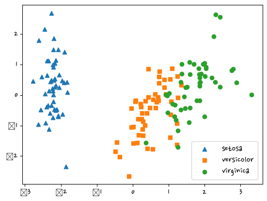
pca.explained_variance_ratio_ #비율확인, 0.72962445전체 변동성의 약 72.9%array([0.72962445, 0.22850762])- 교재 409p
from sklearn.ensemble import RandomForestClassifier
from sklearn.model_selection import cross_val_score
import numpy as np
rcf = RandomForestClassifier(random_state=156)
scores = cross_val_score(rcf,iris.data.iloc[:,:-1],iris.target,scoring='accuracy',cv=3) #scoring = 평가
print(f'개별 정확도:{scores}, 평균정확도: {np.mean(scores)}')개별 정확도:[0.98 0.94 0.96], 평균정확도: 0.96rcf = RandomForestClassifier(random_state=156)
scores = cross_val_score(rcf,df_pca.iloc[:,:-1],iris.target,scoring='accuracy',cv=3) #scoring = 평가
print(f'개별 정확도:{scores}, 평균정확도: {np.mean(scores)}')개별 정확도:[0.88 0.88 0.88], 평균정확도: 0.88from sklearn.datasets import fetch_openmlmnist = fetch_openml('mnist_784')컬러이미지는 기본적으로 3차원이다. 2차원 데이터를 하나로 펼쳐놔서 한 건당 한 행에 해당된다. 가로세로 28픽셀x28픽셀=784
type(mnist)sklearn.utils.Bunchmnist.keys()dict_keys(['data', 'target', 'frame', 'categories', 'feature_names', 'target_names', 'DESCR', 'details', 'url'])mnist.data| pixel1 | pixel2 | pixel3 | pixel4 | pixel5 | pixel6 | pixel7 | pixel8 | pixel9 | pixel10 | ... | pixel775 | pixel776 | pixel777 | pixel778 | pixel779 | pixel780 | pixel781 | pixel782 | pixel783 | pixel784 | |
|---|---|---|---|---|---|---|---|---|---|---|---|---|---|---|---|---|---|---|---|---|---|
| 0 | 0.0 | 0.0 | 0.0 | 0.0 | 0.0 | 0.0 | 0.0 | 0.0 | 0.0 | 0.0 | ... | 0.0 | 0.0 | 0.0 | 0.0 | 0.0 | 0.0 | 0.0 | 0.0 | 0.0 | 0.0 |
| 1 | 0.0 | 0.0 | 0.0 | 0.0 | 0.0 | 0.0 | 0.0 | 0.0 | 0.0 | 0.0 | ... | 0.0 | 0.0 | 0.0 | 0.0 | 0.0 | 0.0 | 0.0 | 0.0 | 0.0 | 0.0 |
| 2 | 0.0 | 0.0 | 0.0 | 0.0 | 0.0 | 0.0 | 0.0 | 0.0 | 0.0 | 0.0 | ... | 0.0 | 0.0 | 0.0 | 0.0 | 0.0 | 0.0 | 0.0 | 0.0 | 0.0 | 0.0 |
| 3 | 0.0 | 0.0 | 0.0 | 0.0 | 0.0 | 0.0 | 0.0 | 0.0 | 0.0 | 0.0 | ... | 0.0 | 0.0 | 0.0 | 0.0 | 0.0 | 0.0 | 0.0 | 0.0 | 0.0 | 0.0 |
| 4 | 0.0 | 0.0 | 0.0 | 0.0 | 0.0 | 0.0 | 0.0 | 0.0 | 0.0 | 0.0 | ... | 0.0 | 0.0 | 0.0 | 0.0 | 0.0 | 0.0 | 0.0 | 0.0 | 0.0 | 0.0 |
| ... | ... | ... | ... | ... | ... | ... | ... | ... | ... | ... | ... | ... | ... | ... | ... | ... | ... | ... | ... | ... | ... |
| 69995 | 0.0 | 0.0 | 0.0 | 0.0 | 0.0 | 0.0 | 0.0 | 0.0 | 0.0 | 0.0 | ... | 0.0 | 0.0 | 0.0 | 0.0 | 0.0 | 0.0 | 0.0 | 0.0 | 0.0 | 0.0 |
| 69996 | 0.0 | 0.0 | 0.0 | 0.0 | 0.0 | 0.0 | 0.0 | 0.0 | 0.0 | 0.0 | ... | 0.0 | 0.0 | 0.0 | 0.0 | 0.0 | 0.0 | 0.0 | 0.0 | 0.0 | 0.0 |
| 69997 | 0.0 | 0.0 | 0.0 | 0.0 | 0.0 | 0.0 | 0.0 | 0.0 | 0.0 | 0.0 | ... | 0.0 | 0.0 | 0.0 | 0.0 | 0.0 | 0.0 | 0.0 | 0.0 | 0.0 | 0.0 |
| 69998 | 0.0 | 0.0 | 0.0 | 0.0 | 0.0 | 0.0 | 0.0 | 0.0 | 0.0 | 0.0 | ... | 0.0 | 0.0 | 0.0 | 0.0 | 0.0 | 0.0 | 0.0 | 0.0 | 0.0 | 0.0 |
| 69999 | 0.0 | 0.0 | 0.0 | 0.0 | 0.0 | 0.0 | 0.0 | 0.0 | 0.0 | 0.0 | ... | 0.0 | 0.0 | 0.0 | 0.0 | 0.0 | 0.0 | 0.0 | 0.0 | 0.0 | 0.0 |
70000 rows × 784 columns
mnist.data.shape(70000, 784)mnist.target.shape(70000,)mnist.target0 5
1 0
2 4
3 1
4 9
..
69995 2
69996 3
69997 4
69998 5
69999 6
Name: class, Length: 70000, dtype: category
Categories (10, object): ['0', '1', '2', '3', ..., '6', '7', '8', '9']mnist.target.value_counts()1 7877
7 7293
3 7141
2 6990
9 6958
0 6903
6 6876
8 6825
4 6824
5 6313
Name: class, dtype: int64mnist.data.min().min()0.0mnist.data.max().max()255.0한 픽셀은 1바이트 = 8비트 = 256개(0-255) 표현가능
0-255값 차이가 많이 나서 값을 0~1 사이로 맞춰줌
from sklearn.ensemble import RandomForestClassifier
from sklearn.model_selection import train_test_split
from sklearn.metrics import accuracy_scoreX_train,X_test,y_train,y_test = train_test_split(mnist.data,mnist.target,test_size=0.1)y_train.value_counts() #대략 나눠짐1 7091
7 6573
3 6459
2 6320
9 6265
6 6209
0 6184
8 6132
4 6106
5 5661
Name: class, dtype: int64#모델생성
clf = RandomForestClassifier()
clf.fit(X_train,y_train)
pred = clf.predict(X_test)
accuracy_score(y_test,pred)0.9724285714285714입력되는 값은 학습데이터랑 같아야 한다? -> 손글씨는 그림이 있어야 한다.
rgb는 흔히 빛의 삼원색이라고 한다. 0=검정, 255=흰색
숫자로 만들 때 검은 바탕에 흰글자여야 한다.


import matplotlib.pyplot as plt
import numpy as np
tmp = X_test.iloc[2]
tmp = np.array(tmp)
tmp = tmp.reshape(28,28)
plt.imshow(tmp,cmap='gray')
y_test.iloc[0]'4'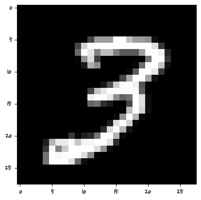
tmparray([[ 0., 0., 0., 0., 0., 0., 0., 0., 0., 0., 0.,
0., 0., 0., 0., 0., 0., 0., 0., 0., 0., 0.,
0., 0., 0., 0., 0., 0.],
[ 0., 0., 0., 0., 0., 0., 0., 0., 0., 0., 0.,
0., 0., 0., 0., 0., 0., 0., 0., 0., 0., 0.,
0., 0., 0., 0., 0., 0.],
[ 0., 0., 0., 0., 0., 0., 0., 0., 0., 0., 0.,
0., 0., 0., 0., 0., 0., 0., 0., 0., 0., 0.,
0., 0., 0., 0., 0., 0.],
[ 0., 0., 0., 0., 0., 0., 0., 0., 0., 0., 0.,
0., 0., 0., 0., 0., 0., 0., 0., 0., 0., 0.,
0., 0., 0., 0., 0., 0.],
[ 0., 0., 0., 0., 0., 0., 0., 0., 0., 0., 0.,
0., 0., 57., 136., 196., 181., 15., 0., 0., 0., 0.,
0., 0., 0., 0., 0., 0.],
[ 0., 0., 0., 0., 0., 0., 0., 0., 0., 0., 0.,
0., 148., 250., 254., 254., 254., 139., 0., 0., 0., 0.,
0., 0., 0., 0., 0., 0.],
[ 0., 0., 0., 0., 0., 0., 0., 0., 0., 0., 1.,
108., 252., 254., 247., 92., 232., 153., 0., 0., 0., 0.,
0., 0., 0., 0., 0., 0.],
[ 0., 0., 0., 0., 0., 0., 0., 0., 0., 0., 111.,
254., 254., 207., 22., 0., 226., 247., 25., 0., 0., 0.,
0., 0., 0., 0., 0., 0.],
[ 0., 0., 0., 0., 0., 0., 0., 0., 0., 44., 250.,
254., 204., 23., 0., 79., 252., 254., 136., 0., 0., 0.,
0., 0., 0., 0., 0., 0.],
[ 0., 0., 0., 0., 0., 0., 0., 0., 6., 167., 254.,
247., 26., 0., 0., 89., 154., 249., 240., 134., 0., 0.,
0., 0., 0., 0., 0., 0.],
[ 0., 0., 0., 0., 0., 0., 0., 0., 76., 254., 254.,
137., 0., 0., 0., 0., 0., 97., 225., 206., 0., 0.,
0., 0., 0., 0., 0., 0.],
[ 0., 0., 0., 0., 0., 0., 0., 3., 185., 254., 235.,
3., 0., 0., 0., 0., 0., 0., 34., 220., 122., 0.,
0., 0., 0., 0., 0., 0.],
[ 0., 0., 0., 0., 0., 0., 0., 56., 254., 254., 109.,
0., 0., 0., 0., 0., 0., 0., 0., 97., 237., 9.,
0., 0., 0., 0., 0., 0.],
[ 0., 0., 0., 0., 0., 0., 0., 104., 254., 218., 12.,
0., 0., 0., 0., 0., 0., 0., 0., 30., 236., 176.,
4., 0., 0., 0., 0., 0.],
[ 0., 0., 0., 0., 0., 0., 0., 105., 254., 207., 0.,
0., 0., 0., 0., 0., 0., 0., 0., 0., 114., 255.,
9., 0., 0., 0., 0., 0.],
[ 0., 0., 0., 0., 0., 0., 0., 174., 254., 206., 0.,
0., 0., 0., 0., 0., 0., 0., 0., 0., 30., 254.,
107., 0., 0., 0., 0., 0.],
[ 0., 0., 0., 0., 0., 0., 0., 104., 254., 206., 0.,
0., 0., 0., 0., 0., 0., 0., 0., 0., 19., 254.,
197., 0., 0., 0., 0., 0.],
[ 0., 0., 0., 0., 0., 0., 0., 104., 254., 206., 0.,
0., 0., 0., 0., 0., 0., 0., 0., 0., 19., 254.,
197., 0., 0., 0., 0., 0.],
[ 0., 0., 0., 0., 0., 0., 0., 104., 254., 250., 44.,
0., 0., 0., 0., 0., 0., 0., 0., 0., 72., 254.,
179., 0., 0., 0., 0., 0.],
[ 0., 0., 0., 0., 0., 0., 0., 62., 254., 254., 165.,
0., 0., 0., 0., 0., 0., 0., 0., 36., 211., 254.,
61., 0., 0., 0., 0., 0.],
[ 0., 0., 0., 0., 0., 0., 0., 7., 225., 254., 248.,
147., 35., 0., 0., 0., 0., 35., 114., 248., 254., 225.,
6., 0., 0., 0., 0., 0.],
[ 0., 0., 0., 0., 0., 0., 0., 0., 62., 228., 254.,
254., 248., 245., 210., 186., 235., 249., 254., 254., 193., 6.,
0., 0., 0., 0., 0., 0.],
[ 0., 0., 0., 0., 0., 0., 0., 0., 0., 39., 210.,
254., 254., 254., 254., 254., 254., 254., 235., 155., 7., 0.,
0., 0., 0., 0., 0., 0.],
[ 0., 0., 0., 0., 0., 0., 0., 0., 0., 0., 5.,
66., 156., 205., 183., 160., 145., 66., 22., 0., 0., 0.,
0., 0., 0., 0., 0., 0.],
[ 0., 0., 0., 0., 0., 0., 0., 0., 0., 0., 0.,
0., 0., 0., 0., 0., 0., 0., 0., 0., 0., 0.,
0., 0., 0., 0., 0., 0.],
[ 0., 0., 0., 0., 0., 0., 0., 0., 0., 0., 0.,
0., 0., 0., 0., 0., 0., 0., 0., 0., 0., 0.,
0., 0., 0., 0., 0., 0.],
[ 0., 0., 0., 0., 0., 0., 0., 0., 0., 0., 0.,
0., 0., 0., 0., 0., 0., 0., 0., 0., 0., 0.,
0., 0., 0., 0., 0., 0.],
[ 0., 0., 0., 0., 0., 0., 0., 0., 0., 0., 0.,
0., 0., 0., 0., 0., 0., 0., 0., 0., 0., 0.,
0., 0., 0., 0., 0., 0.]])import glob
from PIL import Imagefor path in glob.glob('./img/*.png'):
# print(path) #파일경로이름
img = Image.open(path).convert('L')
#print(img)
plt.imshow(img,cmap='gray')
img = np.resize(img,(1,784))
img = 255.0-(img) #실수값으로 맞춰줬다.
#print(img)
pred = clf.predict(img)
print(pred)
plt.show()['0']
C:\anaconda\lib\site-packages\sklearn\base.py:450: UserWarning: X does not have valid feature names, but RandomForestClassifier was fitted with feature names
warnings.warn(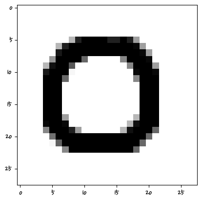
['1']


C:\anaconda\lib\site-packages\sklearn\base.py:450: UserWarning: X does not have valid feature names, but RandomForestClassifier was fitted with feature names
  warnings.warn(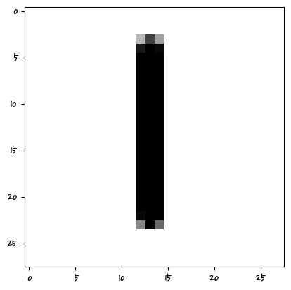
C:\anaconda\lib\site-packages\sklearn\base.py:450: UserWarning: X does not have valid feature names, but RandomForestClassifier was fitted with feature names
  warnings.warn(


['2']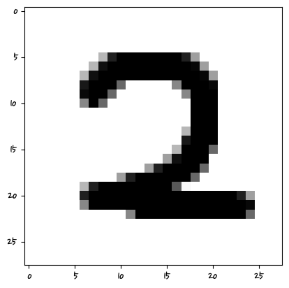
['3']


C:\anaconda\lib\site-packages\sklearn\base.py:450: UserWarning: X does not have valid feature names, but RandomForestClassifier was fitted with feature names
  warnings.warn(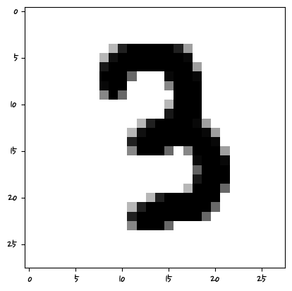
['9']


C:\anaconda\lib\site-packages\sklearn\base.py:450: UserWarning: X does not have valid feature names, but RandomForestClassifier was fitted with feature names
  warnings.warn(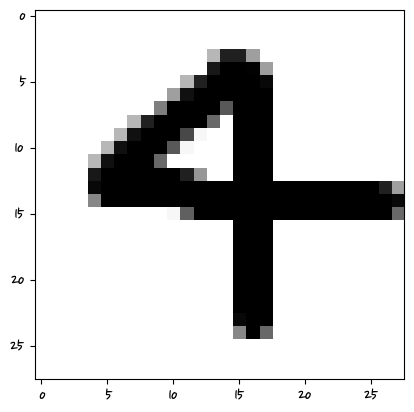
C:\anaconda\lib\site-packages\sklearn\base.py:450: UserWarning: X does not have valid feature names, but RandomForestClassifier was fitted with feature names
  warnings.warn(


['5']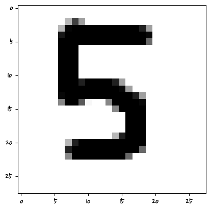
C:\anaconda\lib\site-packages\sklearn\base.py:450: UserWarning: X does not have valid feature names, but RandomForestClassifier was fitted with feature names
  warnings.warn(


['5']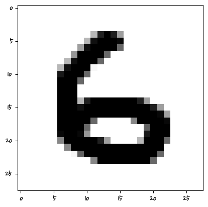
C:\anaconda\lib\site-packages\sklearn\base.py:450: UserWarning: X does not have valid feature names, but RandomForestClassifier was fitted with feature names
  warnings.warn(


['2']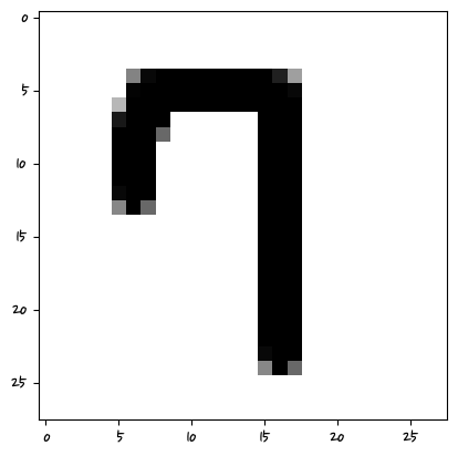
C:\anaconda\lib\site-packages\sklearn\base.py:450: UserWarning: X does not have valid feature names, but RandomForestClassifier was fitted with feature names
  warnings.warn(


['8']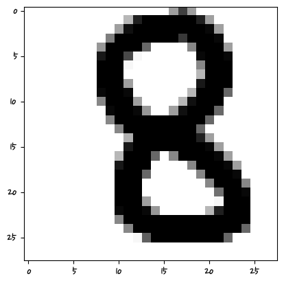
C:\anaconda\lib\site-packages\sklearn\base.py:450: UserWarning: X does not have valid feature names, but RandomForestClassifier was fitted with feature names
  warnings.warn(


['4']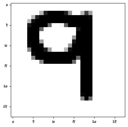
머신러닝은 특성 픽셀의 값을 학습하는 거기 때문에 그 위치에 해당해야 한다.
비정형 데이터는 딥러닝쪽에서 하는 것이 좋다.
log1p적용된 데이터면 입력한 데이터도 log1p가 적용되어야 한다.
학습에 쓰인 데이터 형태와 같은 데이터 형태를 입력해야 제대로 학습할 수 있다.
모델 학습 저장하는 것(pickle)