타이타닉에 대한 예제는 어느정도 진행했으므로 이번엔 <Porto Seguro's Safe Driver Prediction> 에 대해 공부해보려 한다.
https://www.kaggle.com/c/porto-seguro-safe-driver-prediction
먼저 이유한님의 커리큘럼에서 첫 번째 노트북인 <Data Preparation & Exploration> 을 보려한다. 이 노트북은 Bert Carremans이 3년 전에 작성하였고, 2021년 1월 12일 기준 42,118회 의 조회수와 366표 의 투표를 받은 노트북이다.
https://www.kaggle.com/bertcarremans/data-preparation-exploration
Introduction
이 노트북은 결과 도출이 목적이 아닌 데이터 모델링을 위한 팁을 제공한다고 생각하면 된다. 노트북의 주요 섹션은 아래와 같다.
- Visual inspection of your data
- Defining the metadata
- Descriptive statistics
- Handling imbalanced classes
- Data quality checks
- Exploratory data visualization
- Feature engineering
- Feature selection
- Feature scaling
Dataset
Loading Packages
import pandas as pd # 0.25.1
import numpy as np # 1.18.5
import matplotlib.pyplot as plt # 3.2.2
import seaborn as sns # 0.10.1
# scikit-learn 0.23.1
from sklearn.impute import SimpleImputer
from sklearn.preprocessing import PolynomialFeatures, StandardScaler
from sklearn.feature_selection import VarianceThreshold, SelectFromModel
from sklearn.utils import shuffle
from sklearn.ensemble import RandomForestClassifier

import warnings
warnings.filterwarnings('ignore')

pd.set_option('display.max_columns', 100) # 표를 출력할 때 최대 열 수를 설정
Loading data
train = pd.read_csv('train.csv')
test = pd.read_csv('test.csv')
Data at first sight
Kaggle 데이터 설명에 대한 발췌:
- 유사한 그룹에 속하는 피쳐는 피쳐 이름(eg. ind, reg, car, calc)에서와 같이 태그가 지정된다.
- bin은 이진 피쳐, cat은 카테고리 피쳐를 의미한다.
- 이러한 이름이 지정되어 있지 않으면 연속형이거나 순서형 피쳐이다.
- -1은 누락된 값이다.
- target 칼럼은 클레임이 접수되었는지의 여부를 나타낸다.
먼저 이 정보들을 알아보기 위해 head를 이용해서 확인해보자.
train.head()| id | target | ps_ind_01 | ps_ind_02_cat | ps_ind_03 | ps_ind_04_cat | ps_ind_05_cat | ps_ind_06_bin | ps_ind_07_bin | ps_ind_08_bin | ps_ind_09_bin | ps_ind_10_bin | ps_ind_11_bin | ps_ind_12_bin | ps_ind_13_bin | ps_ind_14 | ps_ind_15 | ps_ind_16_bin | ps_ind_17_bin | ps_ind_18_bin | ps_reg_01 | ps_reg_02 | ps_reg_03 | ps_car_01_cat | ps_car_02_cat | ps_car_03_cat | ps_car_04_cat | ps_car_05_cat | ps_car_06_cat | ps_car_07_cat | ps_car_08_cat | ps_car_09_cat | ps_car_10_cat | ps_car_11_cat | ps_car_11 | ps_car_12 | ps_car_13 | ps_car_14 | ps_car_15 | ps_calc_01 | ps_calc_02 | ps_calc_03 | ps_calc_04 | ps_calc_05 | ps_calc_06 | ps_calc_07 | ps_calc_08 | ps_calc_09 | ps_calc_10 | ps_calc_11 | ps_calc_12 | ps_calc_13 | ps_calc_14 | ps_calc_15_bin | ps_calc_16_bin | ps_calc_17_bin | ps_calc_18_bin | ps_calc_19_bin | ps_calc_20_bin | |
|---|---|---|---|---|---|---|---|---|---|---|---|---|---|---|---|---|---|---|---|---|---|---|---|---|---|---|---|---|---|---|---|---|---|---|---|---|---|---|---|---|---|---|---|---|---|---|---|---|---|---|---|---|---|---|---|---|---|---|---|
| 0 | 7 | 0 | 2 | 2 | 5 | 1 | 0 | 0 | 1 | 0 | 0 | 0 | 0 | 0 | 0 | 0 | 11 | 0 | 1 | 0 | 0.7 | 0.2 | 0.718070 | 10 | 1 | -1 | 0 | 1 | 4 | 1 | 0 | 0 | 1 | 12 | 2 | 0.400000 | 0.883679 | 0.370810 | 3.605551 | 0.6 | 0.5 | 0.2 | 3 | 1 | 10 | 1 | 10 | 1 | 5 | 9 | 1 | 5 | 8 | 0 | 1 | 1 | 0 | 0 | 1 |
| 1 | 9 | 0 | 1 | 1 | 7 | 0 | 0 | 0 | 0 | 1 | 0 | 0 | 0 | 0 | 0 | 0 | 3 | 0 | 0 | 1 | 0.8 | 0.4 | 0.766078 | 11 | 1 | -1 | 0 | -1 | 11 | 1 | 1 | 2 | 1 | 19 | 3 | 0.316228 | 0.618817 | 0.388716 | 2.449490 | 0.3 | 0.1 | 0.3 | 2 | 1 | 9 | 5 | 8 | 1 | 7 | 3 | 1 | 1 | 9 | 0 | 1 | 1 | 0 | 1 | 0 |
| 2 | 13 | 0 | 5 | 4 | 9 | 1 | 0 | 0 | 0 | 1 | 0 | 0 | 0 | 0 | 0 | 0 | 12 | 1 | 0 | 0 | 0.0 | 0.0 | -1.000000 | 7 | 1 | -1 | 0 | -1 | 14 | 1 | 1 | 2 | 1 | 60 | 1 | 0.316228 | 0.641586 | 0.347275 | 3.316625 | 0.5 | 0.7 | 0.1 | 2 | 2 | 9 | 1 | 8 | 2 | 7 | 4 | 2 | 7 | 7 | 0 | 1 | 1 | 0 | 1 | 0 |
| 3 | 16 | 0 | 0 | 1 | 2 | 0 | 0 | 1 | 0 | 0 | 0 | 0 | 0 | 0 | 0 | 0 | 8 | 1 | 0 | 0 | 0.9 | 0.2 | 0.580948 | 7 | 1 | 0 | 0 | 1 | 11 | 1 | 1 | 3 | 1 | 104 | 1 | 0.374166 | 0.542949 | 0.294958 | 2.000000 | 0.6 | 0.9 | 0.1 | 2 | 4 | 7 | 1 | 8 | 4 | 2 | 2 | 2 | 4 | 9 | 0 | 0 | 0 | 0 | 0 | 0 |
| 4 | 17 | 0 | 0 | 2 | 0 | 1 | 0 | 1 | 0 | 0 | 0 | 0 | 0 | 0 | 0 | 0 | 9 | 1 | 0 | 0 | 0.7 | 0.6 | 0.840759 | 11 | 1 | -1 | 0 | -1 | 14 | 1 | 1 | 2 | 1 | 82 | 3 | 0.316070 | 0.565832 | 0.365103 | 2.000000 | 0.4 | 0.6 | 0.0 | 2 | 2 | 6 | 3 | 10 | 2 | 12 | 3 | 1 | 1 | 3 | 0 | 0 | 0 | 1 | 1 | 0 |
변수의 특징:
- 이진 변수
- 정수로 되어있는 카테고리형 변수
- 정수형이나 실수형으로된 변수
- -1의 값을 가진 변수
- target과 id
train.shape(595212, 59)현재 train 셋에는 59개의 변수와 595212개의 행이 있다. 중복된 행이 있는지 알아보자.
train.drop_duplicates()
train.shape
(595212, 59)중복된 행은 없는 것으로 보인다.
test.shape(892816, 58)test의 변수가 하나 누락된 것을 알 수 있는데 이는 target 변수일 것이다.
train.info()<class 'pandas.core.frame.DataFrame'>
RangeIndex: 595212 entries, 0 to 595211
Data columns (total 59 columns):
id 595212 non-null int64
target 595212 non-null int64
ps_ind_01 595212 non-null int64
ps_ind_02_cat 595212 non-null int64
ps_ind_03 595212 non-null int64
ps_ind_04_cat 595212 non-null int64
ps_ind_05_cat 595212 non-null int64
ps_ind_06_bin 595212 non-null int64
ps_ind_07_bin 595212 non-null int64
ps_ind_08_bin 595212 non-null int64
ps_ind_09_bin 595212 non-null int64
ps_ind_10_bin 595212 non-null int64
ps_ind_11_bin 595212 non-null int64
ps_ind_12_bin 595212 non-null int64
ps_ind_13_bin 595212 non-null int64
ps_ind_14 595212 non-null int64
ps_ind_15 595212 non-null int64
ps_ind_16_bin 595212 non-null int64
ps_ind_17_bin 595212 non-null int64
ps_ind_18_bin 595212 non-null int64
ps_reg_01 595212 non-null float64
ps_reg_02 595212 non-null float64
ps_reg_03 595212 non-null float64
ps_car_01_cat 595212 non-null int64
ps_car_02_cat 595212 non-null int64
ps_car_03_cat 595212 non-null int64
ps_car_04_cat 595212 non-null int64
ps_car_05_cat 595212 non-null int64
ps_car_06_cat 595212 non-null int64
ps_car_07_cat 595212 non-null int64
ps_car_08_cat 595212 non-null int64
ps_car_09_cat 595212 non-null int64
ps_car_10_cat 595212 non-null int64
ps_car_11_cat 595212 non-null int64
ps_car_11 595212 non-null int64
ps_car_12 595212 non-null float64
ps_car_13 595212 non-null float64
ps_car_14 595212 non-null float64
ps_car_15 595212 non-null float64
ps_calc_01 595212 non-null float64
ps_calc_02 595212 non-null float64
ps_calc_03 595212 non-null float64
ps_calc_04 595212 non-null int64
ps_calc_05 595212 non-null int64
ps_calc_06 595212 non-null int64
ps_calc_07 595212 non-null int64
ps_calc_08 595212 non-null int64
ps_calc_09 595212 non-null int64
ps_calc_10 595212 non-null int64
ps_calc_11 595212 non-null int64
ps_calc_12 595212 non-null int64
ps_calc_13 595212 non-null int64
ps_calc_14 595212 non-null int64
ps_calc_15_bin 595212 non-null int64
ps_calc_16_bin 595212 non-null int64
ps_calc_17_bin 595212 non-null int64
ps_calc_18_bin 595212 non-null int64
ps_calc_19_bin 595212 non-null int64
ps_calc_20_bin 595212 non-null int64
dtypes: float64(10), int64(49)
memory usage: 267.9 MB현재 _cat이 붙은 변수가 14개가 있고, 이를 나중에 더미 변수를 생성해줄 수 있을 것이다. _bin이 붙은 변수는 이미 이진 변수이므로 더미 변수를 생성할 필요는 없다.
데이터는 49개의 정수형 데이터와 10개의 실수형 데이터로 되어있고, Null 값은 -1로 대체되어 없는 것을 확인할 수 있다.
Metadata
데이터 관리를 용이하게 하기 위해 변수에 대한 메타 정보를 데이터 프레임에 저장하려한다.
- role: input, ID, target
- level: nominal, interval, ordinal, binary
- keep: True or False
- dtype: int, float, str
data = []
for f in train.columns:
    # Defining the role
    if f =='target':
        role = 'target'
    elif f == 'id':
        role = 'id'
    else:
        role = 'input'

    # Defining the level
    if 'bin' in f or f == 'target':
        level = 'binary'
    elif 'cat' in f or f =='id':
        level = 'nominal'
    elif train[f].dtype == float:
        level = 'interval'
    elif train[f].dtype == int:
        level = 'ordinal'

    # Initialize keep to True for all variables except for id
    keep = True
    if f == 'id':
        keep = False

    # Defining the data type
    dtype = train[f].dtype

    # Creating a Dict that contains all the metadata for the variable
    f_dict = {
        'varname': f,
        'role': role,
        'level': level,
        'keep': keep,
        'dtype': dtype
    }
    data.append(f_dict)

meta = pd.DataFrame(data, columns=['varname', 'role', 'level', 'keep', 'dtype'])
meta.set_index('varname', inplace=True)
meta| role | level | keep | dtype | |
|---|---|---|---|---|
| varname | ||||
| id | id | nominal | False | int64 |
| target | target | binary | True | int64 |
| ps_ind_01 | input | ordinal | True | int64 |
| ps_ind_02_cat | input | nominal | True | int64 |
| ps_ind_03 | input | ordinal | True | int64 |
| ps_ind_04_cat | input | nominal | True | int64 |
| ps_ind_05_cat | input | nominal | True | int64 |
| ps_ind_06_bin | input | binary | True | int64 |
| ps_ind_07_bin | input | binary | True | int64 |
| ps_ind_08_bin | input | binary | True | int64 |
| ps_ind_09_bin | input | binary | True | int64 |
| ps_ind_10_bin | input | binary | True | int64 |
| ps_ind_11_bin | input | binary | True | int64 |
| ps_ind_12_bin | input | binary | True | int64 |
| ps_ind_13_bin | input | binary | True | int64 |
| ps_ind_14 | input | ordinal | True | int64 |
| ps_ind_15 | input | ordinal | True | int64 |
| ps_ind_16_bin | input | binary | True | int64 |
| ps_ind_17_bin | input | binary | True | int64 |
| ps_ind_18_bin | input | binary | True | int64 |
| ps_reg_01 | input | interval | True | float64 |
| ps_reg_02 | input | interval | True | float64 |
| ps_reg_03 | input | interval | True | float64 |
| ps_car_01_cat | input | nominal | True | int64 |
| ps_car_02_cat | input | nominal | True | int64 |
| ps_car_03_cat | input | nominal | True | int64 |
| ps_car_04_cat | input | nominal | True | int64 |
| ps_car_05_cat | input | nominal | True | int64 |
| ps_car_06_cat | input | nominal | True | int64 |
| ps_car_07_cat | input | nominal | True | int64 |
| ps_car_08_cat | input | nominal | True | int64 |
| ps_car_09_cat | input | nominal | True | int64 |
| ps_car_10_cat | input | nominal | True | int64 |
| ps_car_11_cat | input | nominal | True | int64 |
| ps_car_11 | input | ordinal | True | int64 |
| ps_car_12 | input | interval | True | float64 |
| ps_car_13 | input | interval | True | float64 |
| ps_car_14 | input | interval | True | float64 |
| ps_car_15 | input | interval | True | float64 |
| ps_calc_01 | input | interval | True | float64 |
| ps_calc_02 | input | interval | True | float64 |
| ps_calc_03 | input | interval | True | float64 |
| ps_calc_04 | input | ordinal | True | int64 |
| ps_calc_05 | input | ordinal | True | int64 |
| ps_calc_06 | input | ordinal | True | int64 |
| ps_calc_07 | input | ordinal | True | int64 |
| ps_calc_08 | input | ordinal | True | int64 |
| ps_calc_09 | input | ordinal | True | int64 |
| ps_calc_10 | input | ordinal | True | int64 |
| ps_calc_11 | input | ordinal | True | int64 |
| ps_calc_12 | input | ordinal | True | int64 |
| ps_calc_13 | input | ordinal | True | int64 |
| ps_calc_14 | input | ordinal | True | int64 |
| ps_calc_15_bin | input | binary | True | int64 |
| ps_calc_16_bin | input | binary | True | int64 |
| ps_calc_17_bin | input | binary | True | int64 |
| ps_calc_18_bin | input | binary | True | int64 |
| ps_calc_19_bin | input | binary | True | int64 |
| ps_calc_20_bin | input | binary | True | int64 |
예를 들어 nominal 데이터를 아래처럼 추출할 수 있다.
meta[(meta.level == 'nominal') & (meta.keep)].indexIndex(['ps_ind_02_cat', 'ps_ind_04_cat', 'ps_ind_05_cat', 'ps_car_01_cat',
'ps_car_02_cat', 'ps_car_03_cat', 'ps_car_04_cat', 'ps_car_05_cat',
'ps_car_06_cat', 'ps_car_07_cat', 'ps_car_08_cat', 'ps_car_09_cat',
'ps_car_10_cat', 'ps_car_11_cat'],
dtype='object', name='varname')role, level에 따른 갯수도 구해볼 수 있다.
pd.DataFrame({'count': meta.groupby(['role', 'level'])['role'].size()}).reset_index()| role | level | count | |
|---|---|---|---|
| 0 | id | nominal | 1 |
| 1 | input | binary | 17 |
| 2 | input | interval | 10 |
| 3 | input | nominal | 14 |
| 4 | input | ordinal | 16 |
| 5 | target | binary | 1 |
Descriptive Statistics
생성해둔 메타데이터로 기술 통계를 구하기 수월하다.
Interval Variables
v = meta[(meta.level == 'interval') & (meta.keep)].index
train[v].describe()| ps_reg_01 | ps_reg_02 | ps_reg_03 | ps_car_12 | ps_car_13 | ps_car_14 | ps_car_15 | ps_calc_01 | ps_calc_02 | ps_calc_03 | |
|---|---|---|---|---|---|---|---|---|---|---|
| count | 595212.000000 | 595212.000000 | 595212.000000 | 595212.000000 | 595212.000000 | 595212.000000 | 595212.000000 | 595212.000000 | 595212.000000 | 595212.000000 |
| mean | 0.610991 | 0.439184 | 0.551102 | 0.379945 | 0.813265 | 0.276256 | 3.065899 | 0.449756 | 0.449589 | 0.449849 |
| std | 0.287643 | 0.404264 | 0.793506 | 0.058327 | 0.224588 | 0.357154 | 0.731366 | 0.287198 | 0.286893 | 0.287153 |
| min | 0.000000 | 0.000000 | -1.000000 | -1.000000 | 0.250619 | -1.000000 | 0.000000 | 0.000000 | 0.000000 | 0.000000 |
| 25% | 0.400000 | 0.200000 | 0.525000 | 0.316228 | 0.670867 | 0.333167 | 2.828427 | 0.200000 | 0.200000 | 0.200000 |
| 50% | 0.700000 | 0.300000 | 0.720677 | 0.374166 | 0.765811 | 0.368782 | 3.316625 | 0.500000 | 0.400000 | 0.500000 |
| 75% | 0.900000 | 0.600000 | 1.000000 | 0.400000 | 0.906190 | 0.396485 | 3.605551 | 0.700000 | 0.700000 | 0.700000 |
| max | 0.900000 | 1.800000 | 4.037945 | 1.264911 | 3.720626 | 0.636396 | 3.741657 | 0.900000 | 0.900000 | 0.900000 |
reg variables:
- ps_reg_03 만이 결측값을 가지고 있다.
- min~max의 범위가 다른데 이 부분은 이용할 분류기에 따라 스케일링(StandardScaler)이 필요할 것으로 보인다.
car variables:
- ps_car_12, ps_car_14 에 결측값이 있다.
- min~max의 범위가 달라 스케일링을 고려해봐야한다.
calc variables:
- 결측값이 없다.
- 최댓값이 0.9로 보인다.
- 세 개의 값이 유사한 분포를 보인다.
전체적으로 등간 변수의 범위가 다소 작은데 데이터의 익명화를 위해 변환(log 등)이 이미 적용되었을 수도 있다.
Ordinal Variables
v = meta[(meta.level == 'ordinal') & (meta.keep)].index
train[v].describe()| ps_ind_01 | ps_ind_03 | ps_ind_14 | ps_ind_15 | ps_car_11 | ps_calc_04 | ps_calc_05 | ps_calc_06 | ps_calc_07 | ps_calc_08 | ps_calc_09 | ps_calc_10 | ps_calc_11 | ps_calc_12 | ps_calc_13 | ps_calc_14 | |
|---|---|---|---|---|---|---|---|---|---|---|---|---|---|---|---|---|
| count | 595212.000000 | 595212.000000 | 595212.000000 | 595212.000000 | 595212.000000 | 595212.000000 | 595212.000000 | 595212.000000 | 595212.000000 | 595212.000000 | 595212.000000 | 595212.000000 | 595212.000000 | 595212.000000 | 595212.000000 | 595212.000000 |
| mean | 1.900378 | 4.423318 | 0.012451 | 7.299922 | 2.346072 | 2.372081 | 1.885886 | 7.689445 | 3.005823 | 9.225904 | 2.339034 | 8.433590 | 5.441382 | 1.441918 | 2.872288 | 7.539026 |
| std | 1.983789 | 2.699902 | 0.127545 | 3.546042 | 0.832548 | 1.117219 | 1.134927 | 1.334312 | 1.414564 | 1.459672 | 1.246949 | 2.904597 | 2.332871 | 1.202963 | 1.694887 | 2.746652 |
| min | 0.000000 | 0.000000 | 0.000000 | 0.000000 | -1.000000 | 0.000000 | 0.000000 | 0.000000 | 0.000000 | 2.000000 | 0.000000 | 0.000000 | 0.000000 | 0.000000 | 0.000000 | 0.000000 |
| 25% | 0.000000 | 2.000000 | 0.000000 | 5.000000 | 2.000000 | 2.000000 | 1.000000 | 7.000000 | 2.000000 | 8.000000 | 1.000000 | 6.000000 | 4.000000 | 1.000000 | 2.000000 | 6.000000 |
| 50% | 1.000000 | 4.000000 | 0.000000 | 7.000000 | 3.000000 | 2.000000 | 2.000000 | 8.000000 | 3.000000 | 9.000000 | 2.000000 | 8.000000 | 5.000000 | 1.000000 | 3.000000 | 7.000000 |
| 75% | 3.000000 | 6.000000 | 0.000000 | 10.000000 | 3.000000 | 3.000000 | 3.000000 | 9.000000 | 4.000000 | 10.000000 | 3.000000 | 10.000000 | 7.000000 | 2.000000 | 4.000000 | 9.000000 |
| max | 7.000000 | 11.000000 | 4.000000 | 13.000000 | 3.000000 | 5.000000 | 6.000000 | 10.000000 | 9.000000 | 12.000000 | 7.000000 | 25.000000 | 19.000000 | 10.000000 | 13.000000 | 23.000000 |
- ps_car_11에서만 결측값이 존재한다.
- 범위가 다른 부분들은 스케일링을 해야한다.
Binary Variables
v = meta[(meta.level == 'binary') & (meta.keep)].index
train[v].describe()| target | ps_ind_06_bin | ps_ind_07_bin | ps_ind_08_bin | ps_ind_09_bin | ps_ind_10_bin | ps_ind_11_bin | ps_ind_12_bin | ps_ind_13_bin | ps_ind_16_bin | ps_ind_17_bin | ps_ind_18_bin | ps_calc_15_bin | ps_calc_16_bin | ps_calc_17_bin | ps_calc_18_bin | ps_calc_19_bin | ps_calc_20_bin | |
|---|---|---|---|---|---|---|---|---|---|---|---|---|---|---|---|---|---|---|
| count | 595212.000000 | 595212.000000 | 595212.000000 | 595212.000000 | 595212.000000 | 595212.000000 | 595212.000000 | 595212.000000 | 595212.000000 | 595212.000000 | 595212.000000 | 595212.000000 | 595212.000000 | 595212.000000 | 595212.000000 | 595212.000000 | 595212.000000 | 595212.000000 |
| mean | 0.036448 | 0.393742 | 0.257033 | 0.163921 | 0.185304 | 0.000373 | 0.001692 | 0.009439 | 0.000948 | 0.660823 | 0.121081 | 0.153446 | 0.122427 | 0.627840 | 0.554182 | 0.287182 | 0.349024 | 0.153318 |
| std | 0.187401 | 0.488579 | 0.436998 | 0.370205 | 0.388544 | 0.019309 | 0.041097 | 0.096693 | 0.030768 | 0.473430 | 0.326222 | 0.360417 | 0.327779 | 0.483381 | 0.497056 | 0.452447 | 0.476662 | 0.360295 |
| min | 0.000000 | 0.000000 | 0.000000 | 0.000000 | 0.000000 | 0.000000 | 0.000000 | 0.000000 | 0.000000 | 0.000000 | 0.000000 | 0.000000 | 0.000000 | 0.000000 | 0.000000 | 0.000000 | 0.000000 | 0.000000 |
| 25% | 0.000000 | 0.000000 | 0.000000 | 0.000000 | 0.000000 | 0.000000 | 0.000000 | 0.000000 | 0.000000 | 0.000000 | 0.000000 | 0.000000 | 0.000000 | 0.000000 | 0.000000 | 0.000000 | 0.000000 | 0.000000 |
| 50% | 0.000000 | 0.000000 | 0.000000 | 0.000000 | 0.000000 | 0.000000 | 0.000000 | 0.000000 | 0.000000 | 1.000000 | 0.000000 | 0.000000 | 0.000000 | 1.000000 | 1.000000 | 0.000000 | 0.000000 | 0.000000 |
| 75% | 0.000000 | 1.000000 | 1.000000 | 0.000000 | 0.000000 | 0.000000 | 0.000000 | 0.000000 | 0.000000 | 1.000000 | 0.000000 | 0.000000 | 0.000000 | 1.000000 | 1.000000 | 1.000000 | 1.000000 | 0.000000 |
| max | 1.000000 | 1.000000 | 1.000000 | 1.000000 | 1.000000 | 1.000000 | 1.000000 | 1.000000 | 1.000000 | 1.000000 | 1.000000 | 1.000000 | 1.000000 | 1.000000 | 1.000000 | 1.000000 | 1.000000 | 1.000000 |
- train 세트에서 target의 평균은 3.645%로 아주 불균형한 데이터 세트로 보인다.
- 평균값으로 대부분 0의 값을 가지고 있을 것으로 예상할 수 있다.
Handling Imbalaced Classes
앞서 언급한 것처럼 target이 1인 레코드 비율보다 target이 0인 레코드의 비율이 월등하게 높다. 이렇게하면 예측에 어려움이 있을 수 있으므로, 두 가지 방법 중 한 가지를 적용해서 해결 할 수 있다:
- target = 1 에 대한 오버 샘플링(Oversampling)
- target = 0 에 대한 언더 샘플링(Undersampling)
이 부분의 설명은 예전에 머신러닝 완벽 가이드에서 공부했을 때의 자료를 참고해볼 수 있다. 오버샘플링과 언더샘플링 설명
그 때 언더 샘플링은 "너무 많은 정상 레이블 데이터를 감소시켜 정상 레이블의 경우 오히려 제대로 된 학습을 할 수 없다는 단점이 있어 잘 적용하지 않는다." 라고 했는데 여기선 언더 샘플링을 적용한다.
desired_apriori = 0.10

# target의 인덱스 추출
idx_0 = train[train.target == 0].index
idx_1 = train[train.target == 1].index

# target당 갯수 추출
nb_0 = len(train.loc[idx_0])
nb_1 = len(train.loc[idx_1])

# 언더샘플링 비율 및 target=0의 갯수 계산
undersampling_rate = ((1-desired_apriori) * nb_1)/(nb_0 * desired_apriori)
undersampled_nb_0 = int(undersampling_rate * nb_0)
print(f'Rate to undersample records with target=0: {undersampling_rate}')
print(f'Number of records with target=0 after undersampling: {undersampled_nb_0}')

# 랜덤으로 target=0인 값 추출
undersampled_idx = shuffle(idx_0, random_state=37, n_samples=undersampled_nb_0)

# 리스트 재생성
idx_list = list(undersampled_idx) + list(idx_1)

# 언더샘플링된 데이터 프레임 리턴
train = train.loc[idx_list].reset_index(drop=True)
Rate to undersample records with target=0: 0.34043569687437886
Number of records with target=0 after undersampling: 195246Data Quality Checks
Checking missing values
-1인 값은 결측값을 의미한다.
vars_with_missing = []

for f in train.columns:
    missings = train[train[f] == -1][f].count()
    if missings > 0:
        vars_with_missing.append(f)
        missings_perc = missings/train.shape[0]

        print(f'변수 {f} 는 {missings} 개의 결측값을 가지고 있으며, 퍼센트는 {missings_perc:.2%} 이다.')

print(f'전체 결측값 칼럼 갯수: {len(vars_with_missing)}')
변수 ps_ind_02_cat 는 103 개의 결측값을 가지고 있으며, 퍼센트는 0.05% 이다.
변수 ps_ind_04_cat 는 51 개의 결측값을 가지고 있으며, 퍼센트는 0.02% 이다.
변수 ps_ind_05_cat 는 2256 개의 결측값을 가지고 있으며, 퍼센트는 1.04% 이다.
변수 ps_reg_03 는 38580 개의 결측값을 가지고 있으며, 퍼센트는 17.78% 이다.
변수 ps_car_01_cat 는 62 개의 결측값을 가지고 있으며, 퍼센트는 0.03% 이다.
변수 ps_car_02_cat 는 2 개의 결측값을 가지고 있으며, 퍼센트는 0.00% 이다.
변수 ps_car_03_cat 는 148367 개의 결측값을 가지고 있으며, 퍼센트는 68.39% 이다.
변수 ps_car_05_cat 는 96026 개의 결측값을 가지고 있으며, 퍼센트는 44.26% 이다.
변수 ps_car_07_cat 는 4431 개의 결측값을 가지고 있으며, 퍼센트는 2.04% 이다.
변수 ps_car_09_cat 는 230 개의 결측값을 가지고 있으며, 퍼센트는 0.11% 이다.
변수 ps_car_11 는 1 개의 결측값을 가지고 있으며, 퍼센트는 0.00% 이다.
변수 ps_car_14 는 15726 개의 결측값을 가지고 있으며, 퍼센트는 7.25% 이다.
전체 결측값 칼럼 갯수: 12- ps_car_03_cat 과 ps_car_05_cat은 너무 높은 비중의 결측값이 있으므로 제거한다.
- 카테고리형 변수의 결측값은 -1로 남겨둔다.
- ps_reg_03(countinuous)는 약 18%의 결측값이 있으므로 평균으로 대체한다.
- ps_car_11(ordinal)은 1개의 결측값을 가지고 있으므로 최빈값으로 대체한다.
- ps_car_14(countinuous)는 약 7%의 결측값이 있으므로 평균으로 대체한다.
# 너무 높은 비중의 결측값이 있는 데이터 제거
vars_to_drop = ['ps_car_03_cat', 'ps_car_05_cat']
train.drop(vars_to_drop, inplace=True, axis=1)

# 메타데이터 업데이트
meta.loc[(vars_to_drop), 'keep'] = False

# 평균, 최빈값으로 대체
mean_imp = SimpleImputer(missing_values=-1, strategy='mean')
mode_imp = SimpleImputer(missing_values=-1, strategy='most_frequent')
train['ps_reg_03'] = mean_imp.fit_transform(train[['ps_reg_03']]).ravel()
train['ps_car_14'] = mean_imp.fit_transform(train[['ps_car_14']]).ravel()
train['ps_car_11'] = mode_imp.fit_transform(train[['ps_car_11']]).ravel()
Checking the cardinality of the categorical variables
카테고리형 변수로 더미 변수를 생성하기 전에 각 카테고리 변수에 몇 개의 값들이 있는지 알아보자.
v = meta[(meta.level == 'nominal') & (meta.keep)].index

for f in v:
    dist_values = train[f].value_counts().shape[0]
    print(f'변수 {f} 는 {dist_values} 개의 값을 가지고 있다.')
변수 ps_ind_02_cat 는 5 개의 값을 가지고 있다.
변수 ps_ind_04_cat 는 3 개의 값을 가지고 있다.
변수 ps_ind_05_cat 는 8 개의 값을 가지고 있다.
변수 ps_car_01_cat 는 13 개의 값을 가지고 있다.
변수 ps_car_02_cat 는 3 개의 값을 가지고 있다.
변수 ps_car_04_cat 는 10 개의 값을 가지고 있다.
변수 ps_car_06_cat 는 18 개의 값을 가지고 있다.
변수 ps_car_07_cat 는 3 개의 값을 가지고 있다.
변수 ps_car_08_cat 는 2 개의 값을 가지고 있다.
변수 ps_car_09_cat 는 6 개의 값을 가지고 있다.
변수 ps_car_10_cat 는 3 개의 값을 가지고 있다.
변수 ps_car_11_cat 는 104 개의 값을 가지고 있다.ps_car_11_cat이 많은 값을 가지고 있다. 여기서 필자는 oliver 이 만든 커널을 적용한다.
def add_noise(series, noise_level):
    return series * (1 + noise_level * np.random.randn(len(series)))

def target_encode(trn_series=None, tst_series=None, target=None, min_samples_leaf=1, smoothing=1, noise_level=0):
    '''
    trn_series: train의 카테고리 피쳐(pd.Series)
    tst_series: test의 카테고리 피쳐(pd.Series)
    target: target 데이터(pd.Series)
    min_samples_leaf(int): 카테고리 평균을 고려할 최소 샘플 수
    smoothing(int): 범주형 평균과 이전의 평균의 균형을 유지하는 평활 효과
    '''
    # assert: 가정설정문, 어떤 조건을 테스트하는 디버깅 보조 도구
    assert len(trn_series) == len(target)
    assert trn_series.name == tst_series.name
    temp = pd.concat([trn_series, target], axis=1)
    # target 평균 계산
    averages = temp.groupby(by=trn_series.name)[target.name].agg(['mean', 'count'])
    # smoothing 계산
    smoothing = 1 / (1 + np.exp(-(averages['count'] - min_samples_leaf) / smoothing))
    # 모든 target에 평균 적용
    prior = target.mean()
    # count가 클수록 full_avg가 적게 고려된다.
    averages[target.name] = prior * (1 - smoothing) + averages['mean'] * smoothing
    averages.drop(['mean', 'count'], axis=1, inplace=True)
    # trn에 평균 적용 및 인덱스 복구
    ft_trn_series = pd.merge(trn_series.to_frame(trn_series.name),
                            averages.reset_index().rename(columns={'index': target.name, target.name: 'average'}),
                            on=trn_series.name,
                            how='left')['average'].rename(trn_series.name + '_mean').fillna(prior)
    ft_trn_series.index = trn_series.index
    # tst에 평균 적용 및 인덱스 복구
    ft_tst_series = pd.merge(tst_series.to_frame(tst_series.name),
                            averages.reset_index().rename(columns={'index': target.name, target.name: 'average'}),
                            on=tst_series.name,
                            how='left')['average'].rename(trn_series.name + '_mean').fillna(prior)
    ft_tst_series.index = tst_series.index

return add_noise(ft_trn_series, noise_level), add_noise(ft_tst_series, noise_level)train_encoded, test_encoded = target_encode(train['ps_car_11_cat'],
test['ps_car_11_cat'],
target=train.target,
min_samples_leaf=100,
smoothing=10,
noise_level=0.01)
train['ps_car_11_cat_te'] = train_encoded
train.drop('ps_car_11_cat', axis=1, inplace=True)
meta.loc['ps_car_11_cat', 'keep'] = False
test['ps_car_11_cat_te'] = test_encoded
test.drop('ps_car_11_cat', axis=1, inplace=True)Exploratory Data Visualization
Categorical Variables
카테고리형 변수와 target이 1인 고객의 분포를 확인해보자.
v = meta[(meta.level == 'nominal') & (meta.keep)].index

for f in v:
    plt.figure()
    fig, ax = plt.subplots(figsize=(20, 10))
    cat_perc = train[[f, 'target']].groupby([f], as_index=False).mean()
    cat_perc.sort_values(by='target', ascending=False, inplace=True)
    sns.barplot(ax=ax, x=f, y='target', data=cat_perc, order=cat_perc[f], palette='rocket')
    plt.ylabel('% target', fontsize=18)
    plt.xlabel(f, fontsize=18)
    plt.tick_params(axis='both', which='major', labelsize=18)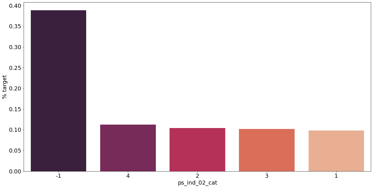
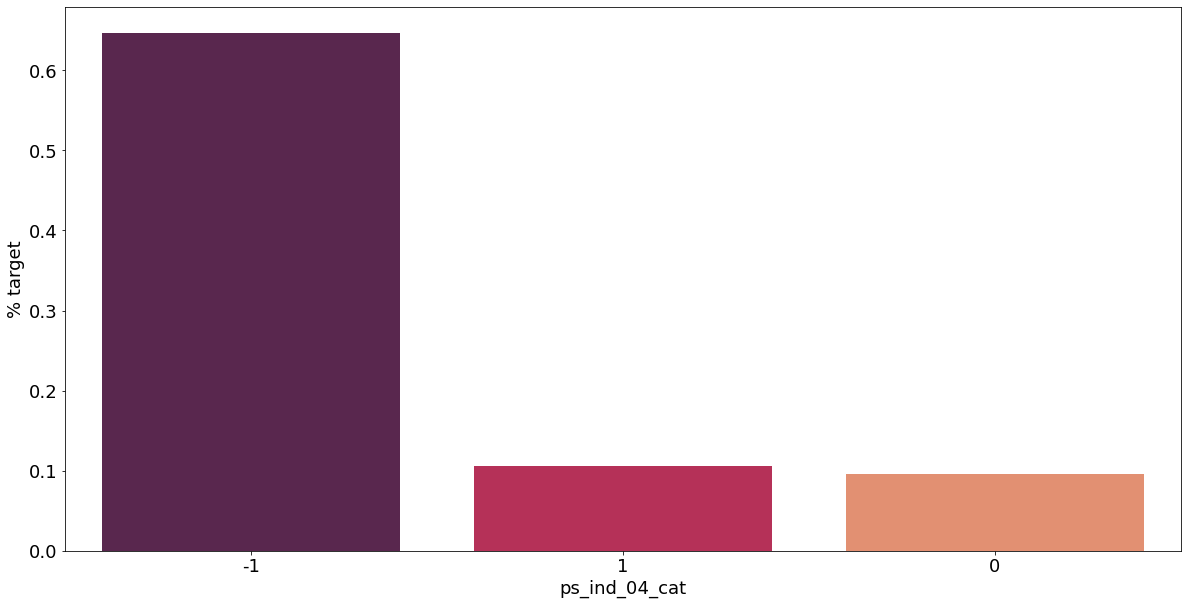
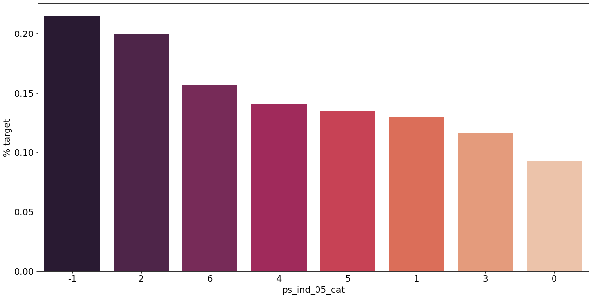
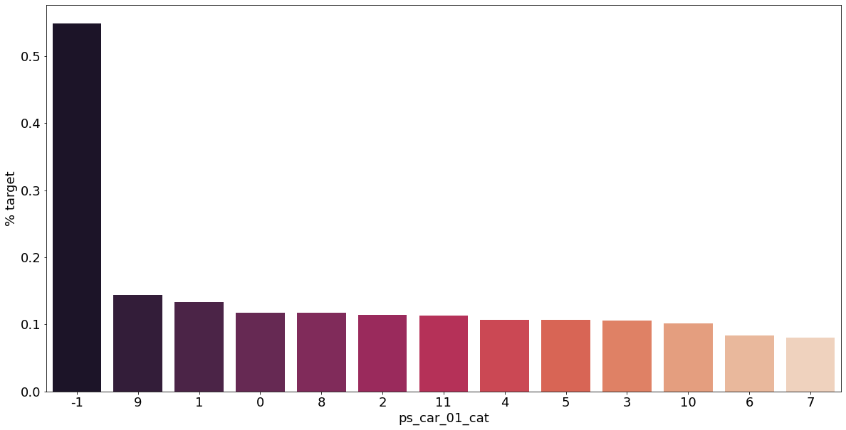
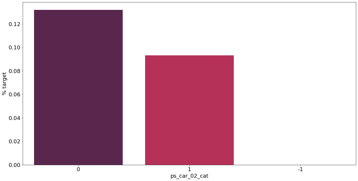
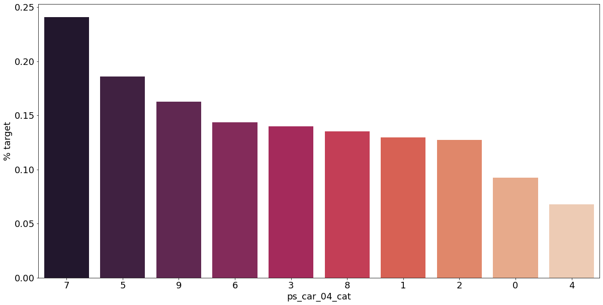
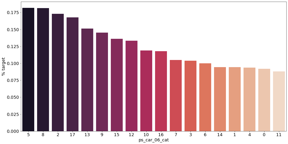
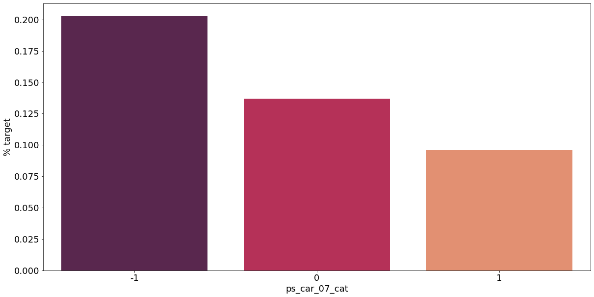
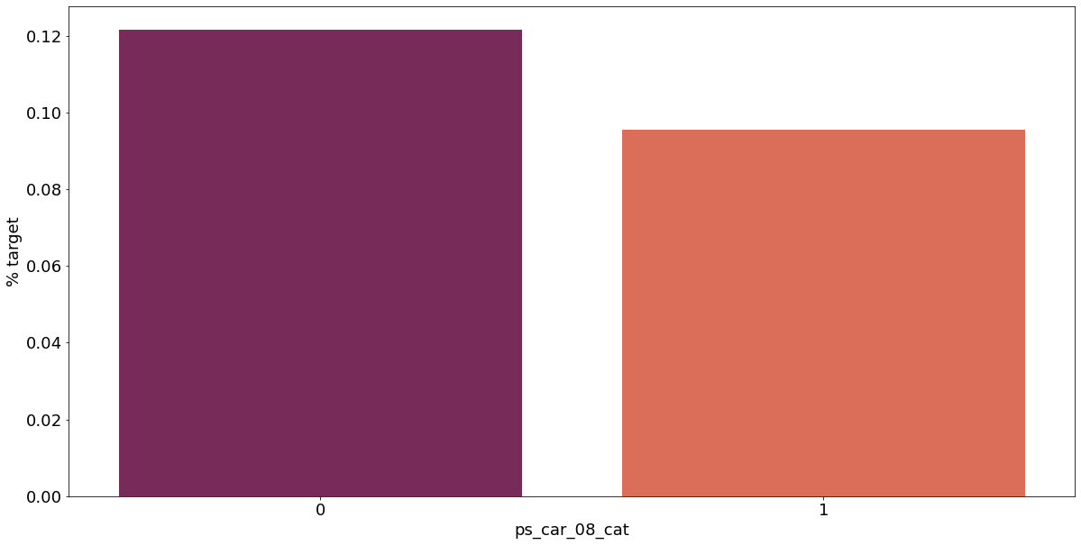
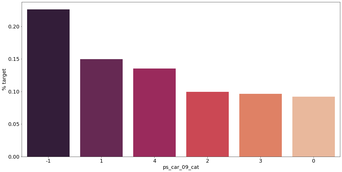

결측값이 있는 고객은 보험 청구를 요청할 확률이 훨씬 높은 것으로 보인다.(낮은 경우도 있음) 이를 최빈값으로 교체하는 등 방법이 다양하게 있을 것이다.
Interval Variables
간격 변수들의 상관 관계를 알아보자. 아래 코드는 an example by Michael Waskom에 기반하여 작성하였다.
def corr_heatmap(v):
    correlations = train[v].corr()

    cmap = sns.diverging_palette(220, 10, as_cmap=True)

    fig, ax = plt.subplots(figsize=(10, 10))
    sns.heatmap(correlations, cmap=cmap, fmt='.2f', square=True, linewidths=.5, annot=True, cbar_kws={'shrink': .75})

v = meta[(meta.level == 'interval') & (meta.keep)].index
corr_heatmap(v)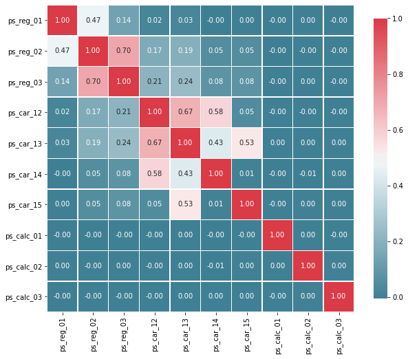
높은 상관관계를 가진 변수들:
- ps_reg_02 와 ps_reg_03 (0.70)
- ps_car_12 와 ps_car_13 (0.67)
- ps_car_12 와 ps_car_14 (0.58)
- ps_car_13 과 ps_car_15 (0.53)
# 빠른 프로세싱을 위해 샘플 추출
s = train.sample(frac=0.1)
ps_reg_02 and ps_reg_03
아래 회귀 직선을 확인하면 피쳐들이 선형 관계가 있다는 것을 알 수 있고, hue 로 회귀 직선이 target=0 일 때와 1일 때를 볼 수 있다.
sns.lmplot('ps_reg_02', 'ps_reg_03', data=s, hue='target', palette='Set1', scatter_kws={'alpha': 0.3})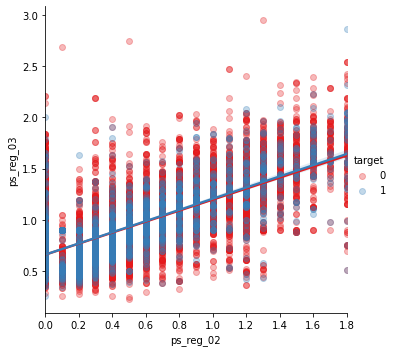
ps_car_12 and ps_car_13
sns.lmplot('ps_car_12', 'ps_car_13', data=s, hue='target', palette='Set2', scatter_kws={'alpha': 0.3})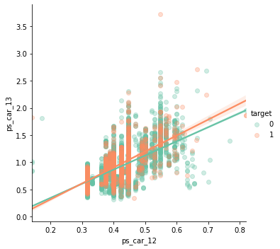
ps_car_12 and ps_car_14
sns.lmplot('ps_car_12', 'ps_car_14', data=s, hue='target', palette='Set3', scatter_kws={'alpha': 0.3})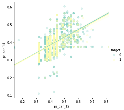
ps_car_13 and ps_car_15
sns.lmplot('ps_car_13', 'ps_car_15', data=s, hue='target', palette='summer_r', scatter_kws={'alpha': 0.3})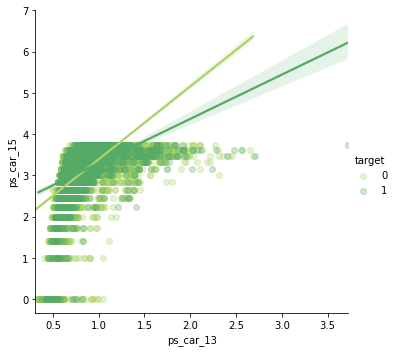
그래프 형태가 더 눈에 띌 수 있게 x, y 축 값을 바꾸자.
sns.lmplot('ps_car_15', 'ps_car_13', data=s, hue='target', palette='winter', scatter_kws={'alpha': 0.3})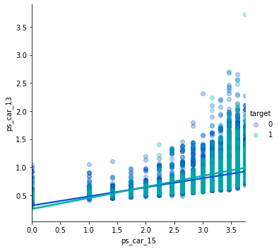
Checking the Correlations between Ordinal Variables
v = meta[(meta.level == 'ordinal') & (meta.keep)].index
corr_heatmap(v)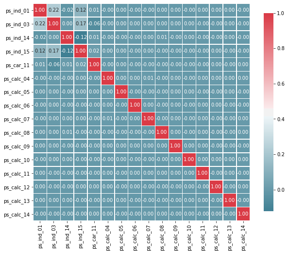
서수형 변수들에선 상관관계가 높게 나타나지 않는다. 하지만 우리는 목표값별로 그룹화할 때 분포가 어떻게 되는지 알아볼 수 있다.
Feature Engineering
Creating Dummy Variables
카테고리형 변수에서 1과 2는 값이 두 배임을 의미하진 않는다. 그러므로 더미형 변수를 만들어줘야 한다. 첫 번째 더미 변수를 삭제하는 이유는 원래 변수의 범주에 대해 생성된 다른 더미 변수에서 파생될 수 있기 때문이다.
v = meta[(meta.level == 'nominal') & (meta.keep)].index
print(f'더미화 전에 train 세트에 있는 변수의 갯수: {train.shape[1]}')
train = pd.get_dummies(train, columns=v, drop_first=True)
print(f'더미화 후에 train 세트에 있는 변수의 갯수: {train.shape[1]}')
더미화 전에 train 세트에 있는 변수의 갯수: 57
더미화 후에 train 세트에 있는 변수의 갯수: 10952개의 더미 변수가 추가되었다.
drop_first에 대한 추가 설명: 타이타닉 예제에서 예를 들면 Pclass가 1, 2, 3이 있었고, 이에 더미 변수를 생성하면 Pclass_1, Pclass_2, Pclass_3이 나온다. 여기서 drop_first 를 하면 Pclass_2, Pclass_3 만 나온다. 이렇게해도 두 값이 0이라면 Pclass가 1임을 알 수 있기 때문이다.
Creating interaction variables
PolynomialFeatures함수는 데이터를 다항식 형태로 변경한다.
- degree: 차수를 조절
- include_bias: True로 할 경우 0차항(1)도 만듦.
- interaction_only: 교호작용을 할 변수만 만들지 여부를 결정.
v = meta[(meta.level == 'interval') & (meta.keep)].index
poly = PolynomialFeatures(degree=2, interaction_only=False, include_bias=False)
interactions = pd.DataFrame(data=poly.fit_transform(train[v]), columns=poly.get_feature_names(v))
interactions.drop(v, axis=1, inplace=True)
print(f'교호작용 전에 train 세트에 있는 변수의 갯수: {train.shape[1]}')
train = pd.concat([train, interactions], axis=1)
print(f'교호작용 후에 train 세트에 있는 변수의 갯수: {train.shape[1]}')
교호작용 전에 train 세트에 있는 변수의 갯수: 109
교호작용 후에 train 세트에 있는 변수의 갯수: 16455개의 교호작용 변수가 추가되었다.
Feature Selection
Removing Features with low or zero variance
분산이 없거나 매우 낮은 피쳐를 제거할 수 있는데, sklearn의 VarianceThreshold 를 이용해서 제거할 수 있다. 기본적으로는 분산이 0인 피쳐를 제거하는데 이전 단계에서 분산이 0인 변수가 없었으므로, 1%미만인 피쳐를 제거하게 설정할 수 있다.
Vectorize는 매트릭스 구조의 데이터의 연산을 일괄적으로 처리할 수 있도록 Series, DataFrame, array 등과 같이 시퀀스형 자료를 함수의 매개변수로 포함시킬 수 있게 하는 것을 말한다.
selector = VarianceThreshold(threshold=0.01)
selector.fit(train.drop(['id', 'target'], axis=1))
f = np.vectorize(lambda x: not x)
v = train.drop(['id', 'target'], axis=1).columns[f(selector.get_support())] # get_support()는 선택된 특성을 boolean 값으로 표시해 어떤 특성이 선택되었는지 확인 가능
print(f'{len(v)} 개의 변수가 너무 낮은 분산을 갖고 있다.')
print(f'변수 리스트:\n{list(v)}')
28 개의 변수가 너무 낮은 분산을 갖고 있다.
변수 리스트:
['ps_ind_10_bin', 'ps_ind_11_bin', 'ps_ind_12_bin', 'ps_ind_13_bin', 'ps_car_12', 'ps_car_14', 'ps_car_11_cat_te', 'ps_ind_05_cat_2', 'ps_ind_05_cat_5', 'ps_car_01_cat_1', 'ps_car_01_cat_2', 'ps_car_04_cat_3', 'ps_car_04_cat_4', 'ps_car_04_cat_5', 'ps_car_04_cat_6', 'ps_car_04_cat_7', 'ps_car_06_cat_2', 'ps_car_06_cat_5', 'ps_car_06_cat_8', 'ps_car_06_cat_12', 'ps_car_06_cat_16', 'ps_car_06_cat_17', 'ps_car_09_cat_4', 'ps_car_10_cat_1', 'ps_car_10_cat_2', 'ps_car_12^2', 'ps_car_12 ps_car_14', 'ps_car_14^2']만약 분산을 바탕으로 선택을 하면 많은 변수가 없어질 수 있다. 그러나 우리가 지금 변수를 많이 갖고있기에 분류기가 선택하도록 하자. sklearn의 SelectFromModel 메서드를 사용하면 최상의 피쳐를 선택하게 할 수 있다. 아래에서 랜덤 포레스트를 통해 방법을 설명한다.
Selecting Features with a Random Forest and SelectFromModel
랜덤 포레스트의 feature importances 를 이용해서 선택하도록 하자. SelectFromModel 로 유지할 변수의 수를 지정할 수 있고, feature importances에 대한 임곗값을 수동으로 설정할 수 있다. 여기선 간단하게 상위 50%만을 설정한다.
이 코드는 GitHub repo of Sebastian Raschka 에서 참고했다.
X_train = train.drop(['id', 'target'], axis=1)
y_train = train['target']

feat_labels = X_train.columns

rf = RandomForestClassifier(n_estimators=1000, random_state=0, n_jobs=-1)
rf.fit(X_train, y_train)
importances = rf.feature_importances_

indices = np.argsort(rf.feature_importances_)[::-1]

for f in range(X_train.shape[1]):
    print("%2d) %-*s %f" % (f + 1, 30, feat_labels[indices[f]], importances[indices[f]]))
1) ps_car_11_cat_te 0.021010
2) ps_car_13 0.017335
3) ps_car_13^2 0.017320
4) ps_car_12 ps_car_13 0.017257
5) ps_car_13 ps_car_14 0.017169
6) ps_reg_03 ps_car_13 0.017106
7) ps_reg_01 ps_car_13 0.016905
8) ps_car_13 ps_car_15 0.016836
9) ps_reg_03 ps_car_14 0.016238
10) ps_reg_03 ps_car_12 0.015469
11) ps_reg_03 ps_car_15 0.015133
12) ps_car_14 ps_car_15 0.015055
13) ps_car_13 ps_calc_02 0.014721
14) ps_car_13 ps_calc_01 0.014721
15) ps_reg_02 ps_car_13 0.014694
16) ps_reg_01 ps_reg_03 0.014691
17) ps_car_13 ps_calc_03 0.014675
18) ps_reg_01 ps_car_14 0.014328
19) ps_reg_03^2 0.014262
20) ps_reg_03 0.014198
21) ps_reg_03 ps_calc_02 0.013798
22) ps_reg_03 ps_calc_03 0.013758
23) ps_reg_03 ps_calc_01 0.013680
24) ps_calc_10 0.013613
25) ps_car_14 ps_calc_02 0.013576
26) ps_car_14 ps_calc_01 0.013515
27) ps_car_14 ps_calc_03 0.013464
28) ps_calc_14 0.013387
29) ps_car_12 ps_car_14 0.012966
30) ps_ind_03 0.012918
31) ps_reg_02 ps_car_14 0.012796
32) ps_car_14^2 0.012751
33) ps_car_14 0.012726
34) ps_calc_11 0.012645
35) ps_reg_02 ps_reg_03 0.012537
36) ps_ind_15 0.012112
37) ps_car_12 ps_car_15 0.010960
38) ps_car_15 ps_calc_03 0.010928
39) ps_car_15 ps_calc_02 0.010836
40) ps_car_15 ps_calc_01 0.010827
41) ps_car_12 ps_calc_01 0.010496
42) ps_calc_13 0.010493
43) ps_car_12 ps_calc_03 0.010317
44) ps_car_12 ps_calc_02 0.010316
45) ps_reg_02 ps_car_15 0.010211
46) ps_reg_01 ps_car_15 0.010167
47) ps_calc_02 ps_calc_03 0.010091
48) ps_calc_01 ps_calc_02 0.010048
49) ps_calc_01 ps_calc_03 0.009998
50) ps_calc_07 0.009883
51) ps_calc_08 0.009807
52) ps_reg_01 ps_car_12 0.009439
53) ps_reg_02 ps_car_12 0.009312
54) ps_reg_02 ps_calc_01 0.009260
55) ps_reg_02 ps_calc_03 0.009243
56) ps_reg_02 ps_calc_02 0.009178
57) ps_reg_01 ps_calc_03 0.009062
58) ps_reg_01 ps_calc_01 0.009057
59) ps_calc_06 0.009052
60) ps_reg_01 ps_calc_02 0.009048
61) ps_calc_09 0.008799
62) ps_ind_01 0.008649
63) ps_calc_05 0.008303
64) ps_calc_04 0.008178
65) ps_calc_12 0.008049
66) ps_reg_01 ps_reg_02 0.008034
67) ps_car_15^2 0.006150
68) ps_car_15 0.006109
69) ps_calc_03^2 0.005977
70) ps_calc_01^2 0.005969
71) ps_calc_03 0.005948
72) ps_calc_01 0.005948
73) ps_calc_02^2 0.005940
74) ps_calc_02 0.005928
75) ps_car_12 0.005318
76) ps_car_12^2 0.005307
77) ps_reg_02 0.004983
78) ps_reg_02^2 0.004959
79) ps_reg_01 0.004173
80) ps_reg_01^2 0.004134
81) ps_car_11 0.003803
82) ps_ind_05_cat_0 0.003586
83) ps_ind_17_bin 0.002851
84) ps_calc_17_bin 0.002687
85) ps_calc_16_bin 0.002609
86) ps_calc_19_bin 0.002552
87) ps_calc_18_bin 0.002487
88) ps_ind_16_bin 0.002409
89) ps_car_01_cat_11 0.002382
90) ps_ind_04_cat_0 0.002370
91) ps_ind_04_cat_1 0.002368
92) ps_car_09_cat_2 0.002325
93) ps_ind_07_bin 0.002312
94) ps_ind_02_cat_1 0.002260
95) ps_car_09_cat_0 0.002093
96) ps_car_01_cat_7 0.002093
97) ps_ind_02_cat_2 0.002089
98) ps_calc_20_bin 0.002056
99) ps_ind_06_bin 0.002051
100) ps_car_06_cat_1 0.001999
101) ps_calc_15_bin 0.001989
102) ps_car_07_cat_1 0.001955
103) ps_ind_08_bin 0.001945
104) ps_car_09_cat_1 0.001820
105) ps_car_06_cat_11 0.001803
106) ps_ind_18_bin 0.001726
107) ps_ind_09_bin 0.001718
108) ps_car_01_cat_10 0.001606
109) ps_car_01_cat_9 0.001598
110) ps_car_06_cat_14 0.001566
111) ps_car_01_cat_6 0.001552
112) ps_car_01_cat_4 0.001550
113) ps_ind_05_cat_6 0.001503
114) ps_ind_02_cat_3 0.001424
115) ps_car_07_cat_0 0.001388
116) ps_car_01_cat_8 0.001356
117) ps_car_02_cat_1 0.001348
118) ps_car_08_cat_1 0.001348
119) ps_car_02_cat_0 0.001308
120) ps_car_06_cat_4 0.001237
121) ps_ind_05_cat_4 0.001217
122) ps_ind_02_cat_4 0.001163
123) ps_car_01_cat_5 0.001145
124) ps_car_06_cat_6 0.001118
125) ps_car_06_cat_10 0.001054
126) ps_car_04_cat_1 0.001046
127) ps_ind_05_cat_2 0.001017
128) ps_car_04_cat_2 0.000991
129) ps_car_06_cat_7 0.000990
130) ps_car_01_cat_3 0.000903
131) ps_car_01_cat_0 0.000877
132) ps_car_09_cat_3 0.000873
133) ps_ind_14 0.000850
134) ps_car_06_cat_15 0.000839
135) ps_car_06_cat_9 0.000807
136) ps_ind_05_cat_1 0.000736
137) ps_car_06_cat_3 0.000696
138) ps_car_10_cat_1 0.000694
139) ps_ind_12_bin 0.000672
140) ps_ind_05_cat_3 0.000667
141) ps_car_09_cat_4 0.000619
142) ps_car_04_cat_8 0.000554
143) ps_car_01_cat_2 0.000549
144) ps_car_06_cat_17 0.000513
145) ps_car_06_cat_16 0.000482
146) ps_car_04_cat_9 0.000435
147) ps_car_06_cat_12 0.000434
148) ps_car_06_cat_13 0.000399
149) ps_car_01_cat_1 0.000391
150) ps_ind_05_cat_5 0.000319
151) ps_car_06_cat_5 0.000285
152) ps_ind_11_bin 0.000210
153) ps_car_04_cat_6 0.000196
154) ps_ind_13_bin 0.000150
155) ps_car_04_cat_3 0.000147
156) ps_car_06_cat_2 0.000138
157) ps_car_06_cat_8 0.000096
158) ps_car_04_cat_5 0.000096
159) ps_car_04_cat_7 0.000085
160) ps_ind_10_bin 0.000075
161) ps_car_10_cat_2 0.000062
162) ps_car_04_cat_4 0.000041sfm = SelectFromModel(rf, threshold='median', prefit=True)
print(f'Selection 전 피쳐의 수: {X_train.shape[1]}')
n_features = sfm.transform(X_train).shape[1]
print(f'Selection 후 피쳐의 수: {n_features}')
selected_vars = list(feat_labels[sfm.get_support()])Selection 전 피쳐의 수: 162
Selection 후 피쳐의 수: 81train = train[selected_vars + ['target']]Feature Scaling
앞서 언급한 것과 같이 train 세트에 standard scaling을 할 수 있고, 이는 몇몇 분류기의 성능을 향상시킬 수 있다.
scaler = StandardScaler()
scaler.fit_transform(train.drop(['target'], axis=1))
array([[-0.45941104, -1.26665356, 1.05087653, ..., -0.72553616,
-1.01071913, -1.06173767],
[ 1.55538958, 0.95034274, -0.63847299, ..., -1.06120876,
-1.01071913, 0.27907892],
[ 1.05168943, -0.52765479, -0.92003125, ..., 1.95984463,
-0.56215309, -1.02449277],
...,
[-0.9631112 , 0.58084336, 0.48776003, ..., -0.46445747,
0.18545696, 0.27907892],
[-0.9631112 , -0.89715418, -1.48314775, ..., -0.91202093,
-0.41263108, 0.27907892],
[-0.45941104, -1.26665356, 1.61399304, ..., 0.28148164,
-0.11358706, -0.72653353]])