https://arxiv.org/abs/1703.06868

Abstract

Gatys 는 바로 style transfer 라고 불리는 새로운 분야를 소개했는데, neural 네트워크로 content image에다가 다른 이미지의 style을 입히는(?) 것입니다. 초반에 나온 방법들은 optimization 과정이 매우 느렸고, 좀 더 발전된 feed-forward neural networks도 소개되었지만 여전히 speed cost가 존재하고 arbitrary한 새로운 스타일에는 적응하지 못한다는 문제가 있습니다.

그래서 이 논문에서는 새로운 adaptive instance normalization (AdaIN) layer를 적용해서 이런 문제를 해결하고자 합니다. Let's dive into paper! 😀

1. Introduction

Gatys는 이미지의 content 와 style 정보 모두를 deep neural networks (DNNs)를 통해 인코딩 할 수 있다는 것을 보여줬습니다. (L. A. Gatys, A. S. Ecker, and M. Bethge. Image style transfer using convolutional neural networks. In CVPR, 2016.)
→ it is possible to change the style of an image while preserving its content.✨
😵 하지만 이 방법은 매우 최적화 과정이 매우매우매우 느리다는 한계점이 있습니다. 이런 한계를 극복하기 위해 stylization을 하나의 forward pass로 수행하는 feed-forward neural networks를 학습시키는 방법이 많이 소개되었는데, 이 방법은 하나의 style에만 국한된다는 (더) 큰 문제가 있었습니다.

그래서 이 논문에서는 최초로!! 이런 flexibility-speed dilemma를 해결해주는 neural style transfer algorithm 을 제안합니다. 👍
논문에서는 이전의 optimization 기반 framework의 flexibility와 feed-forward 방식의 빠른 속도 결과를 결합해서, 실시간으로 arbitrary한 새로운 스타일로 transfer 할 수 있는 방법을 제시합니다. 저자들은 instance normalization (IN) layer 에서 아이디어를 얻어, style normalization 이 좋은 성능을 낸다는 것을 보여줍니다.

논문에서는 IN을 확장해서 adaptive instance normalization (AdaIN) 을 새롭게 제시합니다. 이 방법은 간단하게 content 와 style input 이 주어졌을 때, 두 입력의 평균과 분산을 style input과 동일하도록 조절합니다. (이때, content를 먼저 맞춘 후에 style을 맞춰줍니다.)
그리고 decoder network는 AdaIN output을 다시 image space로 inverting 함으로써 마지막 stylized image를 생성하도록 학습합니다.

이런 AdaIN 방법이 빠르고 flexibility도 유지한다고 저자들은 주장하고 있고 뒤에 실험에서 잘 나와있습니다. 좀 더 살펴봅시다! 😀

2. Related Work

Style transfer

가장 관련이 깊은 주제라고 할 수 있죠. Style Transfer!

1. Optimizaiton Speed 와 Arbitrary Style.

   예전 방법들은 low-level statistics에 의존하고 semantic structures를 잘 파악하지 못하는 문제점이 있었는데, Gatys의 Style transfer이 등장했습니다.👏 DNN의 convolutional layers 에서 feature statistics을 일치시켜서 아주 인상적인 style transfer 결과를 보여줬습니다.

   BUT! 이 프레임워크는 loss 네트워크에서 계산된 content loss와 style loss를 최소화하기 위해 반복적으로 이미지를 업데이트하는 아주 느린 최적화 프로세스를 기반으로 하고 있습니다.

   그래서 이런 최적화 프로세스를 대신해서, 동일한 목적함수를 최소화하도록 학습되는 feed-forward neural network 가 제안되었습니다. 이런 feed-forward style transfer 방법은 최적화가 훨씬 빠르고 실시간 응용이 가능하도록 해줍니다.

   BUT! 이런 feed-forward 방법은 고정된 style에만 fixed 된다는 한계 가 있습니다. 이 한계를 극복하기 위해 몇가지 방법이 소개 되긴 했지만, 여전히 training 중에 관찰되지 않는 임의의 스타일에는 적응할 수 없다는 문제가 있었습니다.

2. Style Loss Function

   두번째로 고려할 사항은 어떤 style loss function 을 사용할 것인지 입니다. Gatys 논문에서는 Gram matrix에 의해 캡처된 feature activations 간의 second-order statistics 을 일치시켜서 style 을 매칭합니다. 다른 방법들로는 MRF loss, adversarial loss, histogram loss, CORAL loss, MMD loss, channel-wise mean 과 variance 사이의 거리 등이 있습니다.

   위의 loss functions은 모두 스타일 이미지와 합성 이미지 간의 일부 feature statistics 를 일치시키는 것을 목표로 하고 있습니다.

Deep generative image modeling.

Image Generation 프레임워크 중에 가장 좋은 visual quality를 자랑하는 GAN은 style transfer 및 cross-domain image generation 에도 적용되고 있습니다.

3. Background

3.1. Batch Normalization

Ioffe and Szegedy 는 feature statistics를 normalizing 해서feed-forward 네트워크가 아주 쉽게 훈련할 수 있게 해주는 batch normalization (BN) layer를 소개했습니다. BN layers는 원래 discriminative 네트워크의 훈련을 가속화할 수 있도록 디자인 되었었는데 generative image modeling 에서도 효과적이라는 것이 밝혀졌습니다.👏

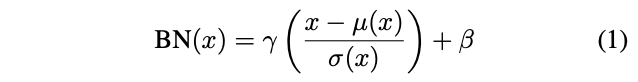
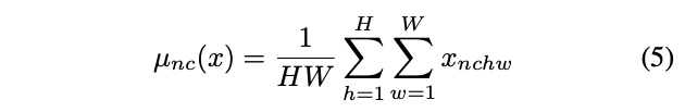
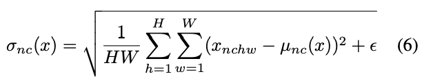
input batch $x ∈ R^{N×C×H×W}$ 가 주어졌을 때, BN 은 각각의 feature channel 에 대해서 평균과 표준편차를 normalize 합니다.
( $γ, β ∈ R^C$: data로 부터 학습된 affine parameters;):

$µ(x), σ(x) ∈ R^C$ 는 평균과 표준편차로, 각 feature channel 에 대해 독립적으로 batch size 및 spatial dimensions 에서 계산됩니다.

3.2. Instance Normalization

원래 feed-forward stylization 방법에서, style transfer network 는 각 convolutional layer 이후에 BN layer를 포함하고 있었습니다.

그런데 Ulyanov가 이 BN layer를 IN layer으로 바꾸는 것이 상당한 성능 향상을 보인다는 것을 발견했습니다. 😀

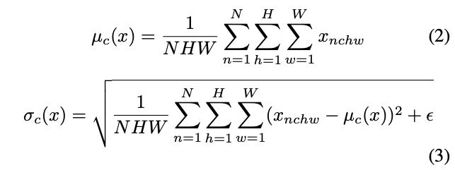
BN layers 와 달리 여기서 $µ(x)$ 와 $σ(x)$는 각각의 channel과 sample에 대해 독립적인 spatial dimensions에서 계산됩니다.:

또다른 차이점 하나는 IN layers는 테스트 시간에 변경되지 않고 적용되는 반면, 일반적으로 BN layers는 minibatch statistics를 population statistics로 대체한다는 것입니다.

3.3. Conditional Instance Normalization

단일의 affine parameters $γ$ 와 $β$ 세트를 학습하는 것 대신에 Dumoulin은 각 스타일마다 별개의 parameters 세트 $γ$ 와 $β$를 학습하는 conditional instance normalization (CIN) layer를 제안했습니다. :

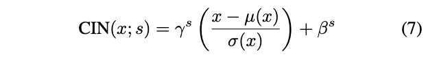
training 중에. style image와 해당하는 indexs가 고정된 style set $s ∈$ {$1, 2, ..., S$}에서 무작위로 선택됩니다.(위 논문 실험에서는 $S = 32$.) 그리고 content image 는 해당 $γ^s$ 와 $β^s$가 CIN layer 에서 사용되는 style transfer network 에 의해 처리됩니다. 진짜 신기한 것은, 네트워크가 IN layers에서 동일한 convolutional parameters를 사용하지만 다른 affine parameters를 사용하기 떄문에 완전히 다른 스타일로 이미지를 생성할 수 있습니다. 👍(WOW)

하지만, normalization layers가 없는 네트워크와 비교해봤을 때, CIN layers가 있는 네트워크는 추가로 $2FS$ parameters가 필요합니다. ($F$ : total number of feature maps in the network.) 추가로 필요한 parameters 수는 styles의 수에 따라 선형으로 확장되기 때문에 많은 수의 styles(e.g.,tens of thousands)을 모델링하도록 방법을 확장하는 것은 어렵습니다. 또한 이런 접근 방식은 네트워크를 re-training 하지 않으면 임의의 새로운 스타일에 적응할 수 없습니다.😭

4. Interpreting Instance Normalization

(conditional) instance normalization 이 잘되는 이유를 한번 알아보자❗️

Ulyanov attribute the success of IN to its invariance to the contrast of the content image. 하지만 IN은 feature space에서 발생하므로, pixel space의 단순한 contrast normalization 보다 더 큰 영향을 미칩니다. 더 놀랄만한 것은 IN의 affine parameters가 출력 이미지의 스타일을 완전히 변경할 수 있다는 사실!!

앞선 연구들이 동기가 되어, 논문에서는 instance normalization가 feature statistics, 즉 평균과 분산을 normalizing 해서 일종의 style normalization 를 수행한다고 주장 합니다.
이전 연구에서는 DNN이 비록 image descriptor 역할을 했었지만, 저자들은 generator network의 feature statistics 또한 생성된 이미지의 style을 제어할 수 있다고 생각합니다.

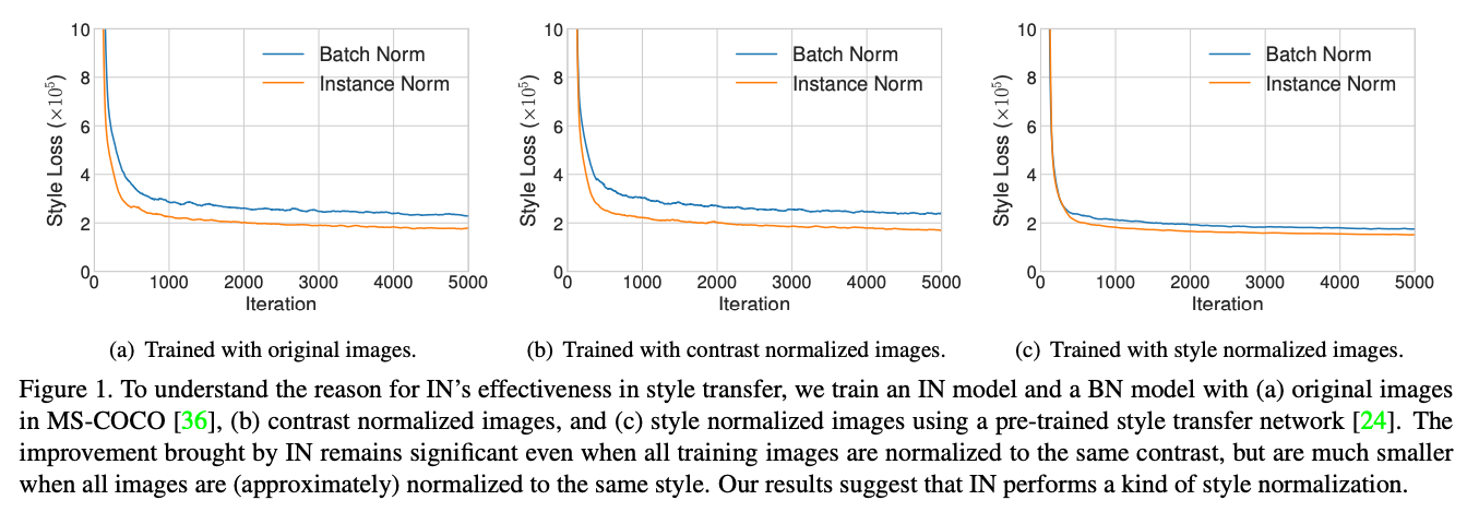
그래서 저자들은 IN or BN layers를 사용해서 single-style transfer을 수행하기 위해 개선된 texture networks 코드를 실행했다고 합니다.

• Fig. 1 (a) : 예상대로, IN이 있는 모델이 BN 보다 빠르게 수렴합니다.
• Fig. 1 (b) : Ulyanov의 설명을 테스트 해보기 위해서, we then normalize all the training images to the same contrast by performing histogram equalization on the luminance channel. → IN은 여전히 effective 하기 때문에, Ulyanov의 설명은 incomplete...
• Fig. 1 (c) : 저자들의 가설을 검증하기 위해서, pretrained 된 style transfer network 를 사용하여 모든 훈련 이미지를 동일한 style(different from the target style)로 정규화합니다. → 이미지가 이미 style normalized 되어 있을 때 IN 으로 인한 개선은 훨씬 작아집니다. (나머지 차이는 pretrained된 네트워크가 완벽하지 않아서...)
• 또한 style normalized images에 대해 훈련된 BN이 있는 모델은 원본 이미지에 대해 훈련된 IN이 있는 모델만큼 빠르게 수렴할 수 있습니다.
  
  Our results indicate that IN does perform a kind of style normalization.

직관적으로, BN은 single sample 이 아닌 samples batch의 feature statistics을 정규화하기 때문에 single style을 중심으로 나머지 batch를 정규화한다고 이해할 수 있습니다. 하지만 각 single sample 에는 서로 다른 스타일이 있을 수 있기 때문에, 모든 이미지를 동일한 style로 transfer 하는 feed-forward style tranfer 알고리즘과 같은 경우는 바람직하지 않습니다. 😢
그리고 비록 convolutional layers은 이것이 가능하다해도, trainig 시간이 오래 걸린다는 추가적인 문제가 있습니다. 😢

반면에, IN은 각 개별 sample의 스타일을 target style로 normalize 할 수 있습니다. 나머지 네트워크는 원본 style information을 버리고 content manipulation 에 집중할 수 있으므로 학습이 용이합니다. 😀

The reason behind the success of CIN also becomes clear: different affine parameters can normalize the feature statistics to different values, thereby normalizing the output image to different styles.

5. Adaptive Instance Normalization

👀 그러면 IN이 affine parameter 로 지정된 single style을 입력으로 normalize하면 adaptive affine transformations 을 사용하여 임의로 지정된 그 스타일에 적용할 수 있을까?
→ Simple Extension to IN, adaptive instance normalization (AdaIN).

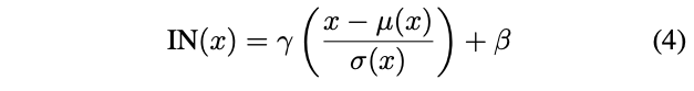
AdaIN은 입력으로 content input $x$ 와 style input $y$를 받고, 간단하게 $x$ 의 channelwise 평균과 분산을 $y$의 것과 일치하도록 조정합니다. BN, IN or CIN 과 다르게, AdaIN은 학습가능한 affine parameters가 없고, 대신 style input에서 affine parameter를 adaptively 하게 계산합니다.: in which we simply scale the normalized content input with $σ(y)$, and shift it with $µ(y)$. Similar to IN, these statistics are computed across spatial locations.

Intuitively, let us consider a feature channel that detects brushstrokes of a certain style. A style image with this kind of strokes will produce a high average activation for this feature. The output produced by AdaIN will have the same high average activation for this feature, while preserving the spatial structure of the content image. The brushstroke feature can be inverted to the image space with a feed-forward decoder. The variance of this feature channel can encoder more subtle style information, which is also transferred to the AdaIN output and the final output image.

짧게 말해서, AdaIN은 feature space에서 channel-wise 로 mean과 variance를 조정하면서 style transfer를 수행합니다.

6. Experimental Setup

6.1. Architecture

6.1. Architecture

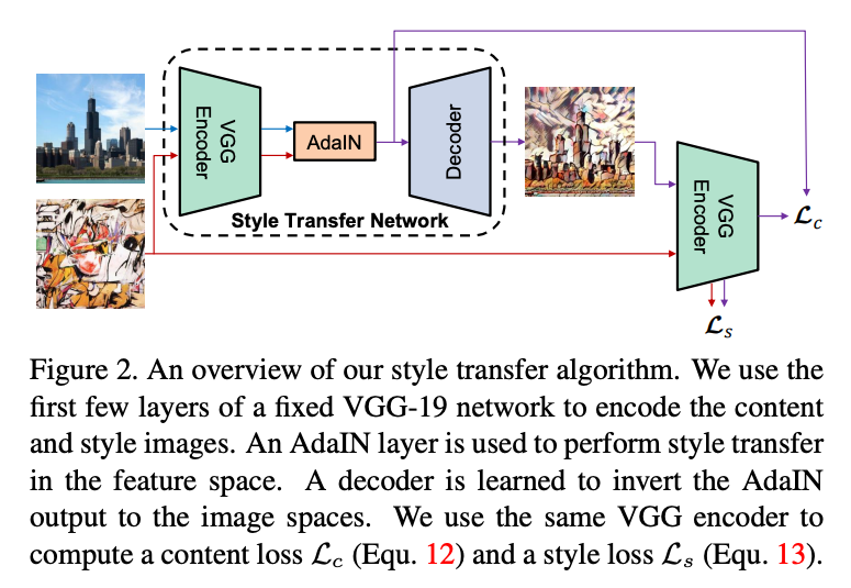
• Style transfer network $T$
• Input
  • content image $c$
  • arbitrary style image $s$

Synthesizes an output image that recombines the content of the former and the style latter.

• encoder $f$ : fixed to pre-trained VGG-19 up to relu4_1.
  

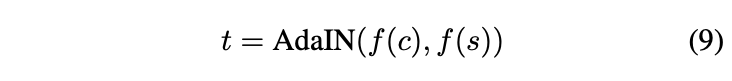
After encoding the content and style images in feature space, we feed both feature maps to an AdaIN layer that aligns the mean and variance of the content feature maps to those of the style feature maps, producing the target feature maps $t$:

• decoder $g$ : randomly initialized and trained to map $t$ back to the image space, generating the stylized image $T(c, s)$:
  

그리고 논문에서는 decoder에서 normalization layers 를 사용하지 않았습니다.

6.2. Training

• Training network ( Each dataset contains roughly 80,000 training examples)
  • MS-COCO : content images
  • WikiArt : style images
• Adam optimizer
• Batch size of 8 content-style image pairs.

Using pre-trained VGG19 to compute the loss function to train the decoder (content loss $L_c$ , style loss $L_s$, style loss weight $λ$)

Content loss : Euclidean distance between target features & features of output image.

We use the AdaIN output $t$ as the content target , instead of feature responses of the content image. Because it is slightly faster convergence and also aligns with our goal of inverting the AdaIN output $t$.

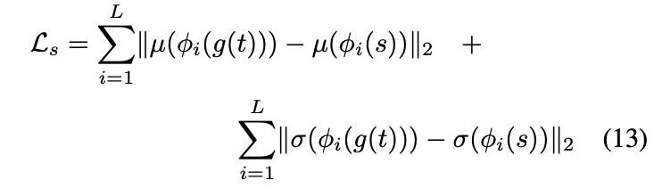
Style loss : only matches these statistics, because AdaIN layer only transfers the mean and standard deviation of the style features.

each $\phi_i$ denotes a layer in VGG-19 used to compute the style loss. In our experiments we use relu1_1, relu2_1, relu3_1, relu4_1 layers with equal weights.

7. Results

7.1. Comparison with other methods

Compare AdaIN approach with three types of style transfer methods:

1. Image style transfer using convolutional neural networks.(flexible but slow optimization)
2. Fast feed-forward method restricted to a single style. (Improved texture networks)
3. Fast patch-based style transfer of arbitrary style. (flexible patch-based method)

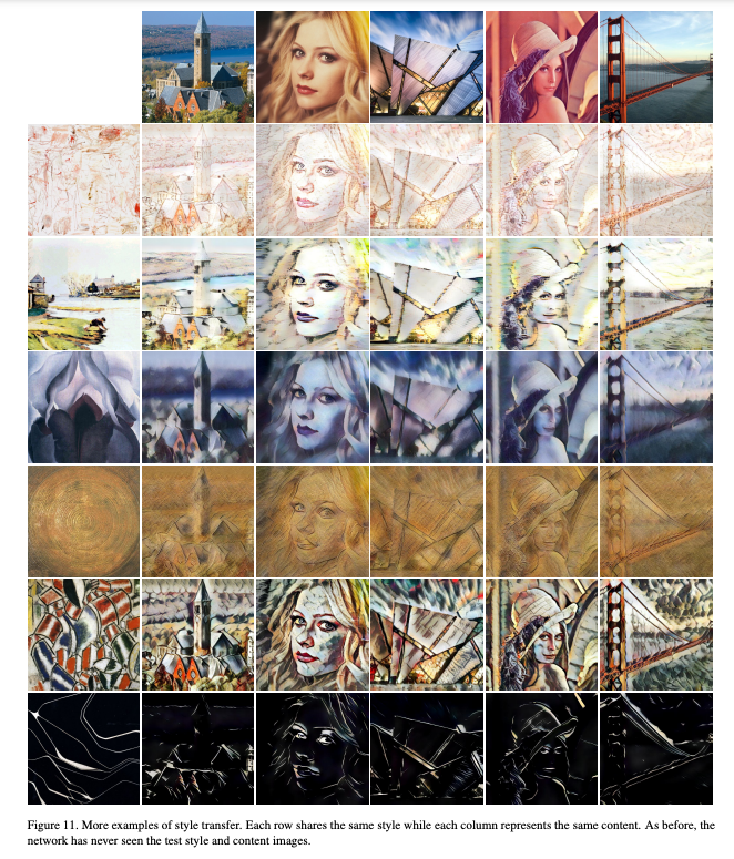
Qualitative Examples.

👀 Note that all the test style images are never observed during the training of our model.

• Even so, the quality of our stylized images is quite competitive with other method in many images (e.g., row 1, 2, 3).
• Compared with ‘Fast feed-forward method’, our method appears to transfer the style more faithfully for most compared images.
  

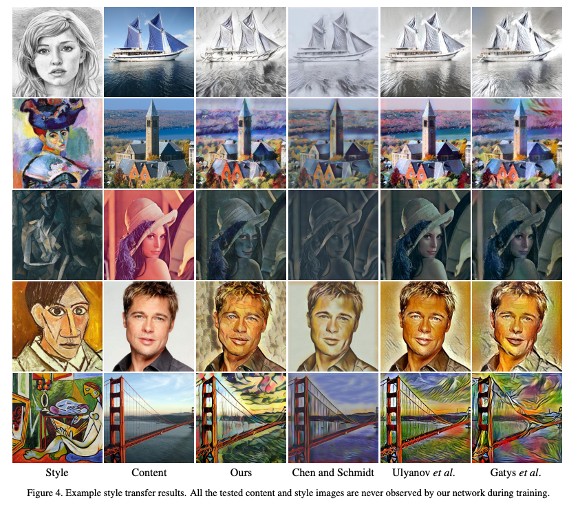
We thus argue that matching global feature statistics is a more general solution, although in some cases (e.g., row 3) the method of ‘Fast feed-forward method’ can also produce appealing results.

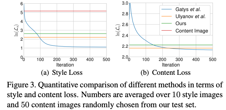
Quantitative evaluations.
We compare our approach with the optimization-based method and the fast single-style transfer method in terms of the content and style loss.

As shown in Fig. 3, the average content and style loss of our synthesized images are slightly higher but comparable to the single-style transfer method of Ulyanov.

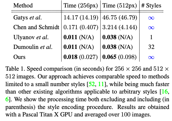
Speed analysis.

In Tab. 1 we compare the speed of our method with previous ones. Excluding the time for style encoding, our algorithm runs at 56 and 15 FPS for 256 × 256 and 512 × 512 images respectively, making it possible to process arbitrary user-uploaded styles in real-time.

7.2. Additional experiments.

7.2. Additional experiments.

• Enc-AdaIN-Dec.
• Enc-Concat-Dec (replaces AdaIN with concatenation)
• Enc-AdaIN-BNDec & Enc-AdaIN-INDec

Verifies that IN layers tend to normalize the output to a single style and thus should be avoided when we want to generate images in different styles. → Enc-Concat-Dec can reach low style loss but fail to decrease the content loss. Models with BN/IN layers also obtain qualitatively worse results and consistently higher losses. The results with IN layers are especially poor.

Verifies our claim that IN layers tend to normalize the output to a single style and thus should be avoided when we want to generate images in different styles. → Verifies our claim that IN layers tend to normalize the output to a single style and thus should be avoided when we want to generate images in different styles.

7.3. Runtime controls

Flexibility of our method, allows users

• to control the degree of stylizatio
• interpolate between different styles
• transfer styles while preserving colors
• use different styles in different spatial regions.

Note that all these controls are only applied at runtime using the same network, without any modification to the training procedure.

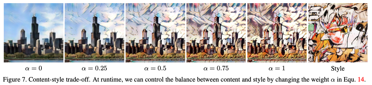
Content-style trade-off.

Degree of style transfer can be controlled during training by adjusting the style weight $λ$ in Equation (11). In addition, our method allows content-style trade-off at test time by interpolating between feature maps that are fed to the decoder.

Smooth transition between content-similarity and style-similarity can be observed by changing $α$ from $0$ to $1$.

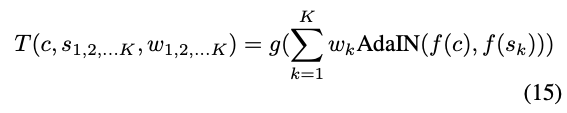
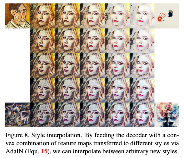
Style interpolation.
To interpolate between a set of $K$ style images $s_1, s_2, ..., s_K$ with corresponding weights $w_1, w_2, ..., w_K$ such that $\sum_{k=1}^{K} w_k = 1$, we similarly interpolate between feature maps:

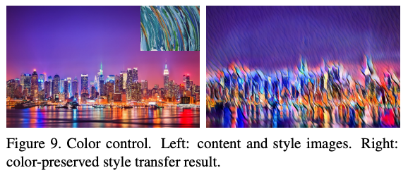
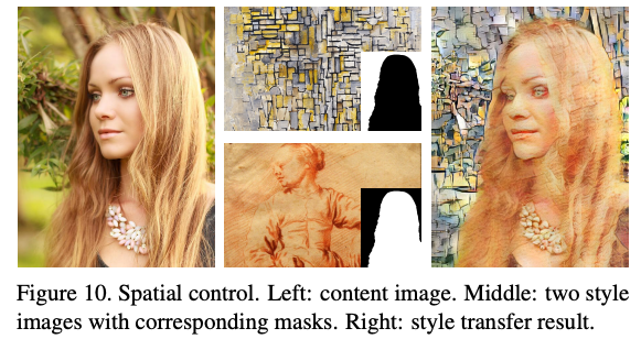
Spatial and color control.
To preserve the color of the content image, we first match the color distribution of the style image to that of the content image, then perform a normal style transfer using the color-aligned style image as the style input.

Our method can transfer different regions of the content image to different styles. This is achieved by performing AdaIN separately to different regions in the content feature maps using statistics from different style inputs.

8. Discussion and Conclusion

• 논문에서는 실시간으로 arbitrary한 style transfer를 가능하게 해주는 adaptive instance normalization (AdaIN) layer를 제안했습니다.
• 이전의 방법들인 Gatys의 optimization process, feed-forward neural networks로 대체한 방법들을 발전시켜서, 논문에서는 statistics을 feature space에서 한방에 조정하고 그 feature를 다시 pixel space로 invert하는 방법을 제시했습니다.
  

Very COOL ✨

Reference

Partial Convolution based Padding

• Zero padding : 가장자리 패딩영역을 0으로 채움
• Reflection padding : 가장자리 기준으로 input값을 패딩영역에 반전하여 복사하여 채움
• Replication padding : 가장자리 근처에 있는 input값을 그대로 복사하여 채움