[U_stage] - week 7

[Day1] 2021/09/13

강의 리뷰

-CV 6강-1: CNN Visualization

• CNN blackbox: low level에서는 방향성이 있는 선이나 블록을 찾고 층이 높아질 수록 의미가 있는 특징을 뽑아낸다.
• Model특성분석:
  • Embedding feature analysis
    - Nearest neighbors in a feature space
    : 의미론적으로 비슷한 concept이 clustering. 물체의 위치변화에 강인하게 학습.
    - Dimensonally reduction
    : 고차원상의 feature를 t-SNE같은 방법을 통해서 차원축소.
  • Activation investigation
    - layer activation: mid와 high layer의 hidden layer의 역할
    - maximally actviation patches
    : 분석하고자하는 층의 채널을 선택 -> 예제 데이터를 backbone에 넣고 activation을 뽑고 저장 -> 가장 큰값의 위치를 파악하고 입력 도메인의 receptive field 계산후 해단 patch crop
    - class visualization: gradient ascent. 임의의 영상(ex.노이즈)의 prediction score -> 타켓 스코어가 최대가 되는 입력을 찾아 gradient update -> current image update -> 반복.
• Model decision explanation
  • saliency test
    - Occlusion map: occlusion map으로 이미지의 일부를 가려 prediction score을 계산 후 관찰.
  • via Backpropagation: 입력 영상을 넣어주고 하나의 class score를 구함 -> 입력도메인까지 얻어진 backprogation후의 gradient를 절대값 취함 -> gradient magnitude map으로 viasualize.
  • Backpropagtion - based saliency
    - Rectified unit(backward pass): backward pass에 relu를 적용.
    - Guided backpropation: forward의 relu패턴과 backward pass에도 relu적용.
  • Class activation mapping
    - class activation mapping(CAM): 어떤 부분을 참조를 하였는지 heatmap처럼 시각화. neural network에서 conv layer와 fc layer사이에 global average pooling을 추가.(단, 성능이 떨어질 수 도 있음)
    - Grad-CAM: 구조를 변경하지않고 재학습없이 CAM을 뽑을 수 있는 방법.
    - SCOUTER: 왜 아닌지도 알 수 있는 비교방법.

[Day2] 2021/09/14

강의 리뷰

-CV 7강: Instance/Panoptic Segmentation and Landmark Localization

• Instance Segmentation
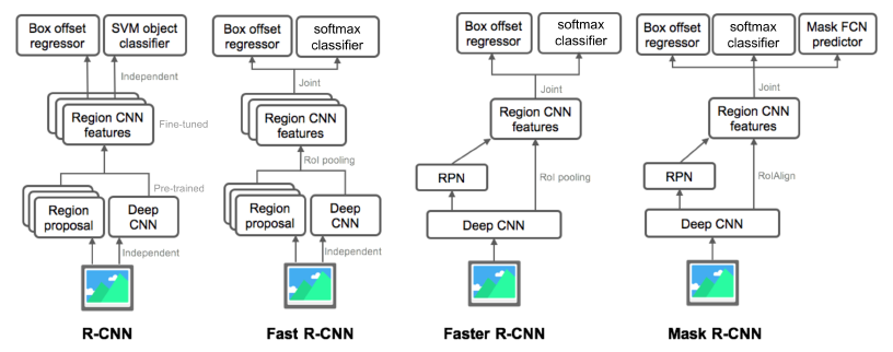
  : semantic segmentation + distinguishing instances
  • Mask R-CNN
    : RoIAlign을 통해서 RoI 추출(interplation을 통해서 정교한 소수점 픽셀레벨). Faster R-CNN + Mask branch.(two stage)
    
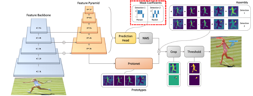
  • YOLACT
    :real time으로(single stage). 기본 backbone으로 feature pyramid구조(고해상도). mask prototype을 생성.
    
  • YolactEdge
    : 소형 디바이스에 적용하기위해 등장. feature map의 계산량을 획기적으로 줄임-> 속도향상.
• Panoptic segmentation
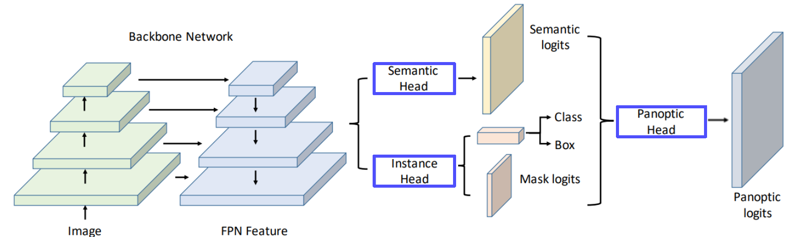
  : stuff + Instances of things.
  • UPSNet
    : semantic & Instance head -> panoptic head -> Panoptic logits
    
  • VPSNet(for video)
    
• Landmark localization
  : keypoint를 정의하고 추정하고 추적
  • coordinate regression: 부정확하고 biased
  • heatmap classification: 좋은 성능, 하지만 높은 계산량.
  • Hourglass network
    : 영상을 작게 만들어 receptive field를 키워
    전반적인 큰 그림을 보아 landmark를 찾는다. skip connection있어 low-level feature로 정확한 위치를 참고. 여러번 반복하여 detail. Unet과도 비슷하지만 FPN이랑도 비슷.
  • DensePose
    : UVmap으로 3D를 2D로 표현. DensePose R-CNN = Faster R-CNN + 3D surface regression branch.
  • RetinaFace
    : FPN + Multi-task branches
• Detecting objects as keypoints
  • CornerNet, CenterNet(1), CenterNet(2).

[Day3] 2021/09/15

강의 리뷰

-CV 8강: Conditional Generative Model

• Conditional Generative model
  : genarative model은 랜덤한 샘플을 만들어 낸다면, conditional generative model은 주어진 조건의 랜덤 샘플을 만들어낸다.
  • ex) style transfer, super resolution, colorization.
  • Super resolution
    : 저해상도 이미지 입력 고해상도 이미지 출력. regrassion은 MAE/MSE로 pixel intensity측정. 그러나 GAN loss는 더 진짜같은 출력.
• Image translation GANs
  • Pix2Pix
    : L1 loss만 사용하면 blurry image를 만들기 때문에, GAN loss로 realistic 이미지 출력.
  • CycleGAN
    : pix2pix는 pairwise data가 필요하지만 현실적으로 쉽지 않음. non-pairwise.
    - CycleGAN loss = GAN loss(in both direction) + Cycle-consistency loss
    - GAN loss만 사용하면 입력과 상관없이 같은 출력. => Cycle-consistency loss (원본 유지)
  • Perceptual loss
    : GAN loss는 train하기 힘들지만 pretrained network는 필요없다. 그러나 perceptual loss는 학습하기 편하고 간단하지만 pretrained network가 필요하다.
• Various GAN applications
  • Deepfake, Face de-identification....

[Day4] 2021/09/16

강의 리뷰

-CV 9강: Multi-modal learning

• 어려운 점:
  • 데이터의 표현방법이 모두 다름 ( 오디오: 1D, 이미지: 2D or 3D,텍스트: embedding vector).
  • feature space의 특징들이 unbalance.
  • 특정 modality에 model이 biased될 수 있음.
• Multi-modal tasks (1)- Visual data & Text
  • Text embedding
    - text embedding: dense vector로 나타냄
    - word2vec: skip-gram model, 주변의 n개의 워드를 predict
  • Joint embedding: matching하기 위한 공통된 embedding vector를 학습하는 방법.
    - Image tagging: pretrained된 unimodal model을 합침. matching의 경우 같은embedding space에 mapping간의 distance를 줄이도록.
    - Image & food recipe retrieval: ingredients/instructions의 순서 -> RNN으로 fixed vector. -> cosine similarity loss & semantic regularization loss
  • Cross modal translation
    - Image captioning: image to sentence(CNN for image, RNN for sentence)
    - show and tell: Encoder (CNN model pre-trained), Decoder(LSTM)
    - show, attend, and tell: 이미지를 입력 -> CNN -> RNN with attention -> word by word generation
    - Text-to-image by generative model: one to many
  • Cross modal reasoning
    - Visual question answering: image stream & question stream을 CNN/RNN으로 embedding vector로 만들고 end-to-end training
• Multi-modal tasks (2) - Visual data & Audio
  • Sound 표현: 1D signal -> acoustic feature로 변환(푸리에 변환 STFT) -> Spectrogram(이미지와 비슷한 형태)
  • Joint embedding
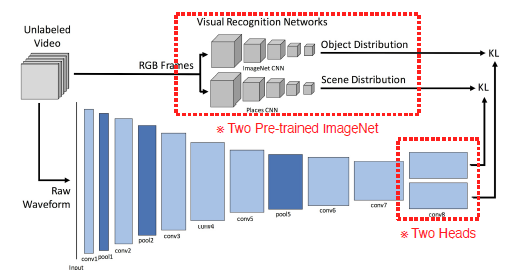
    - Scene regcognition by sound (sound tagging)
    - SoundNet: 비디오 데이터셋의 frame을 labeling되지 않은 상태에서 pretrained Visual Recognition Networks(ImageNet CNN & Places CNN) 사용하여 object distribution과 Scene distribution 출력. 비디오의 오디오는 raw waveform형태로 입력, 1D CNN-> two heads -> 각 distrivution에 KL. pool5 feature를 써서 target task를 할 수 있음.
    
  • Cross modal translation
    - Speech2Face: Module Network(VGG-Face Model사용, Face decoder미리 학습), spectrogram사용.
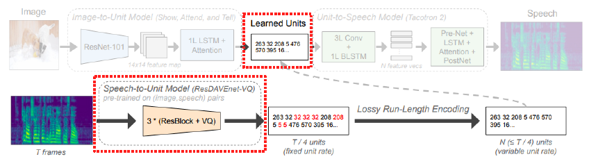
    - Image-to-speech:
    
  • Cross modal reasoning
    - Sound source localization: 소리의 위치object를 찾아냄. visual net과 audio net로 feature를 뽑아 attention net에 다시 입력 => localization score 출력(supervised loss with GT) - fully supervised version.
    - Speech seperation: N detected faces + STFT for spectrogram -> spectrogram mask -> L2 loss(between "clean spectrogram" and "enhanced spectrogram")

[Day5] 2021/09/17

강의 리뷰

-CV 10강: 3D Understanding

• Triangulation: 2D 이미지들로 3D를 만드는 방법.
• 3D data representation: Multi-view images, Volumetric(voxel), Part assembly, Point coud, Mesh(graph CNN), Implicit shape
• 3D datasets
  • ShapeNet: 대량의 가상 3D 이미지
  • PartNet: 디테일한 , segmentation에 유리한.
  • SceneNet: 가상 실내 이미지
  • ScanNet
  • Outdoor: KITTI, Semantic KITTI, Waymo Open Dataset
• 3D task
  • 3D recognition: volumetric CNN 등의 방법.
  • 3D object detection: 이미지나 3D에서 3Dbounding box를 detect.
  • 3D semantic segmentation
  • Mesh R-CNN: 2D를 입력받아 3D detection. 3D brach + Mask RCNN.