1. numerical data visualization
import seaborn as sns

titanic = sns.load_dataset('titanic') # 타이타닉 데이터 불러오기
titanic['alive'][100]titanic.head() # 상위 5개 행만 보여주기| survived | pclass | sex | age | sibsp | parch | fare | embarked | class | who | adult_male | deck | embark_town | alive | alone | |
|---|---|---|---|---|---|---|---|---|---|---|---|---|---|---|---|
| 0 | 0 | 3 | male | 22.0 | 1 | 0 | 7.2500 | S | Third | man | True | NaN | Southampton | no | False |
| 1 | 1 | 1 | female | 38.0 | 1 | 0 | 71.2833 | C | First | woman | False | C | Cherbourg | yes | False |
| 2 | 1 | 3 | female | 26.0 | 0 | 0 | 7.9250 | S | Third | woman | False | NaN | Southampton | yes | True |
| 3 | 1 | 1 | female | 35.0 | 1 | 0 | 53.1000 | S | First | woman | False | C | Southampton | yes | False |
| 4 | 0 | 3 | male | 35.0 | 0 | 0 | 8.0500 | S | Third | man | True | NaN | Southampton | no | True |
1.1 히스토그램(histplot)
print(titanic.size) # 13365개13365
titanic은 dataframe, x축을 age 열로
sns.histplot(data=titanic, x='age');
x축을 age 열인데, 나이대를 10개로 나누기 bin이 10개. 8살 간격
sns.histplot(data=titanic, x='age', bins=10);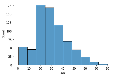
x축을 age 열인데, 나이대를 20개로 나누기 bin이 20개. 4살 간격
sns.histplot(data=titanic, x='age', bins=20);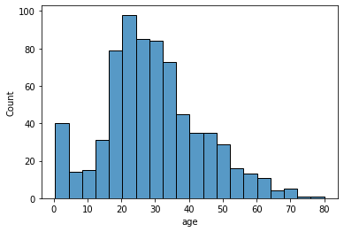
1.1.1 빈도를 특정 categorical data로도 보고 싶을 때.
- 보다시피 생존자 수 그래프와 사망자 수 그래프를 포개지게 그려진다.
- 회색 구간이 두 그래프가 서로 겹친 부분
x축을 age열로, 살았는 지 여부(yes or no)를 hue 값으로
sns.histplot(data=titanic, x='age', hue='alive', bins=4);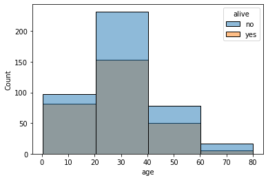
1.1.2 포개지 않고 생존자 수 위에 사망자 수를 누적해 표현하는 방법
multiple='stack'
sns.histplot(data=titanic, x='age', hue='alive', multiple='stack');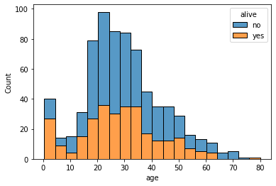
sns.histplot(data=titanic, x='fare', hue='alive', multiple='stack', bins=30);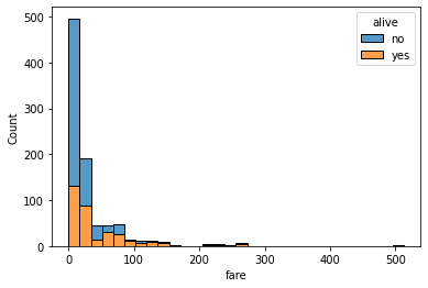
1.2 kernel density estimation function 그래프(kdeplot)
sns.kdeplot(data=titanic, x='fare');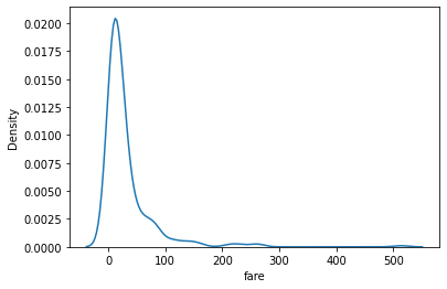
sns.kdeplot(data=titanic, x='age', hue='alive', multiple='stack');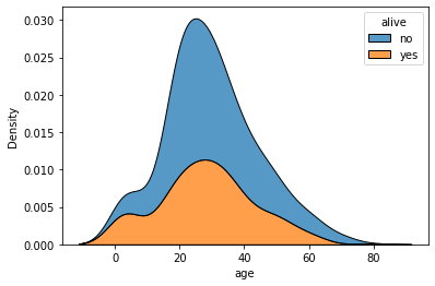
1.3 분포도(displot)
- numerical data 분포를 나타내는 그래프
histplot()과kdeplot()모두 그릴 수 있음
sns.displot(data=titanic, x='age');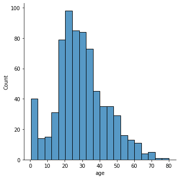
1.3.1 kernel density estimation function
kind=kde
sns.displot(data=titanic, x='age', kind='kde');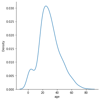
1.3.2 histplot 과 kdeplot 동시에 그리는 법
kde=True
sns.displot(data=titanic, x='age', kde=True);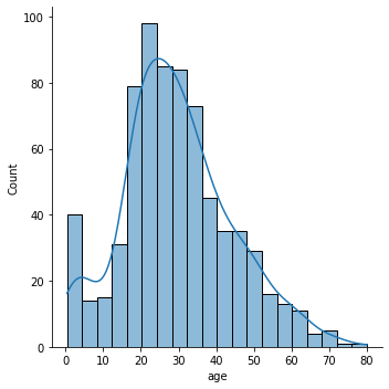
1.4 러그플롯(rugplot)
rugplot은 marginal distribution을 나타내는 그래프.
단독으로 사용하기보다 주로 다른 분포도 그래프와 함께 사용.
다음은 kernel density estimation 함수 그래프와 rugplot을 함께 그린 예시
- age feature가 어떻게 분포돼 있는지 x축 위에 작은 선분으로 표시
- 값이 밀집돼 있을수록 작은 선분들도 밀집
sns.kdeplot(data=titanic, x='age')
sns.rugplot(data=titanic, x='age');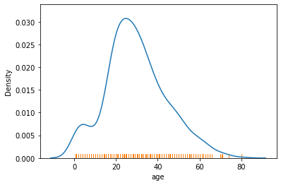
2. Categorical Date Visualization
2.1 barplot
Categorical data 값(x축)에 따라 numerical data 값이 어떻게 달라지는 지 파악할 때 사용
barplot()은 categorical data에 따른 numerical data의 mean, median, max, min과 신뢰구간을 그려줌.
- numerical data의 mean은 bar height로
- 신뢰 구간은 error bar로 표현.
원본 data를 복원 샘플링하여 얻은 표본을 활용해 mean과 신뢰구간을 구하는 것.
즉,barplot()은 원본 data 평균이 아니라 sampling한 data평균을 구해줌.신뢰구간이란?
모수가 실제로 포함될 것을 예측하는 범위
https://bioinformaticsandme.tistory.com/256
x에 categorical data, y에 numerical data 전달.
estimator= np.max, np.min, np.median
sns.barplot(data=titanic, x='class', y='fare');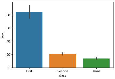
sns.barplot(data=titanic, x='deck', y='fare')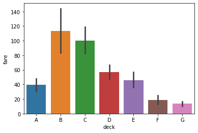
import numpy as npsns.barplot(data=titanic, x='class', y='fare', estimator=np.max);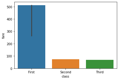
2.2 pointplot
barplot과 동일한 정보 제공.
다만 그래프를 점과 선으로 나타냄.
sns.pointplot(x='class', y='fare', data=titanic);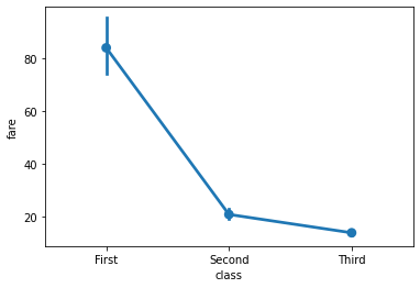
sns.pointplot(x='sex', y='age',hue='deck', data=titanic);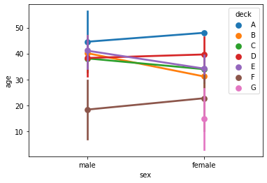
2.3 boxplot
barplot 그래프나 pointplot보다 더 많은 정보를 5가지 요약 수치를 제공
- : 전체 데이터 중 하위 25%에 해당하는 값
- : 50%에 해당하는 값
- : 상위 25%에 해당하는 값
- IQR:
- 최댓값: outlier를 제외하고 가장 큰 값.
- 최솟값: outlier를 제외하고 가장 작은 값.
- outlier: 최댓값보다 큰 값과 최솟값보다 작은 값
sns.boxplot(x='class', y='age', data=titanic);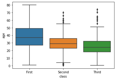
sns.boxplot(x='sex', y='fare', data=titanic);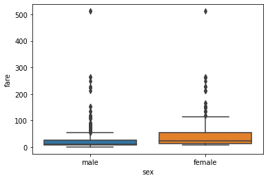
2.4 Violinplot
violin plot은 box plot과 kernel density estimation 함수 그래프를 함쳐 놓은 그래프
- 최솟값, Q1, 중앙값, Q2, 최댓값, 이상치 모두 포함
sns.violinplot(data=titanic, x='class', y='fare');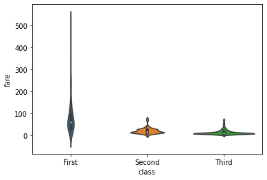
sns.violinplot(data=titanic, x='sex', y='age');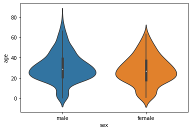
2.5 countplot
categorical data의 빈도(개수)를 확인할 때 사용하는 그래프
range data 구간별이나 categorical에 따른 분포를 파악하기 위해 사용
barplot과 달리 x feature만 전달하면 됨.
sns.countplot(x='class', data=titanic);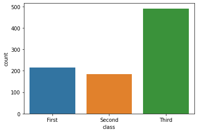
sns.countplot(x='sex', data=titanic);
2.7 pie 그래프
categorical data 비율이 비슷하지 않을 때 한눈에 알아볼 수 있는 그래프
seaborn에서는 지원하지 않아 matplotlib이 필요함
import matplotlib.pyplot as plt

x = [10, 60, 30]
labels = ['A','B', 'C']

# %.1f%% -> %.1f 소수점 첫째 자리, %% %문자 붙이기

#plt.pie(x=x, labels=labels, autopct="%.1f%%");

z= [2,4,8]
z_label=['C','D','E']

plt.pie(x=z, labels=z_label, autopct="%.1f%%");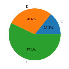
3. data column visualization
3.1 heatmap
data 간 관계를 색상으로 표현한 그래프.
비교해야할 column이 많은 경우 사용
import seaborn as sns

flights = sns.load_dataset('flights')- categorical data 2개(year, month)
- numerical data 1개(passengers)
flights.head()| year | month | passengers | |
|---|---|---|---|
| 0 | 1949 | Jan | 112 |
| 1 | 1949 | Feb | 118 |
| 2 | 1949 | Mar | 132 |
| 3 | 1949 | Apr | 129 |
| 4 | 1949 | May | 121 |
pivot()
index와columns에 전달한 feature를 각각 행과 열로 지정values에 전달한 featrue를 합한 표로 반환
각 연도의 월별 승객 수를 알고 싶으면
year를 index로month를 columns로, 합산할 numerical data는passengers
flights_pivot = flights.pivot(index='year', columns='month', values='passengers')

flights_pivot| month | Jan | Feb | Mar | Apr | May | Jun | Jul | Aug | Sep | Oct | Nov | Dec |
|---|---|---|---|---|---|---|---|---|---|---|---|---|
| year | ||||||||||||
| 1949 | 112 | 118 | 132 | 129 | 121 | 135 | 148 | 148 | 136 | 119 | 104 | 118 |
| 1950 | 115 | 126 | 141 | 135 | 125 | 149 | 170 | 170 | 158 | 133 | 114 | 140 |
| 1951 | 145 | 150 | 178 | 163 | 172 | 178 | 199 | 199 | 184 | 162 | 146 | 166 |
| 1952 | 171 | 180 | 193 | 181 | 183 | 218 | 230 | 242 | 209 | 191 | 172 | 194 |
| 1953 | 196 | 196 | 236 | 235 | 229 | 243 | 264 | 272 | 237 | 211 | 180 | 201 |
| 1954 | 204 | 188 | 235 | 227 | 234 | 264 | 302 | 293 | 259 | 229 | 203 | 229 |
| 1955 | 242 | 233 | 267 | 269 | 270 | 315 | 364 | 347 | 312 | 274 | 237 | 278 |
| 1956 | 284 | 277 | 317 | 313 | 318 | 374 | 413 | 405 | 355 | 306 | 271 | 306 |
| 1957 | 315 | 301 | 356 | 348 | 355 | 422 | 465 | 467 | 404 | 347 | 305 | 336 |
| 1958 | 340 | 318 | 362 | 348 | 363 | 435 | 491 | 505 | 404 | 359 | 310 | 337 |
| 1959 | 360 | 342 | 406 | 396 | 420 | 472 | 548 | 559 | 463 | 407 | 362 | 405 |
| 1960 | 417 | 391 | 419 | 461 | 472 | 535 | 622 | 606 | 508 | 461 | 390 | 432 |
sns.heatmap(data=flights_pivot);
3.2 lineplot
두 numerical data 사이 관계를 나타낼 때
x에 전달한 값에 따라 y에 전달한 값의 평균과 95% 신뢰구간을 나타냄
sns.lineplot(x='year', y='passengers', data=flights);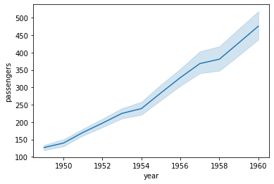
3.4 scatterplot
두 data의 관계를 점으로 표현.
tips = sns.load_dataset('tips')
tips.head()| total_bill | tip | sex | smoker | day | time | size | |
|---|---|---|---|---|---|---|---|
| 0 | 16.99 | 1.01 | Female | No | Sun | Dinner | 2 |
| 1 | 10.34 | 1.66 | Male | No | Sun | Dinner | 3 |
| 2 | 21.01 | 3.50 | Male | No | Sun | Dinner | 3 |
| 3 | 23.68 | 3.31 | Male | No | Sun | Dinner | 2 |
| 4 | 24.59 | 3.61 | Female | No | Sun | Dinner | 4 |
- 총액이 늘면 팁도 증가할 것이다
sns.scatterplot(x='total_bill', y='tip', data=tips);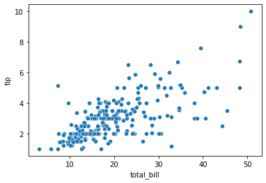
sns.scatterplot(x='total_bill', y='size', hue='sex', data=tips);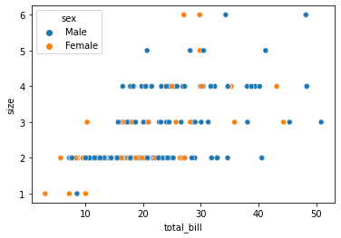
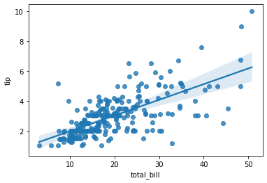
3.5 regplot(회귀선을 포함한 scatterplot)
- scatterplot과 regression line을 동시에 그려줌.
- regression line을 그리면 상관관계 파악이 쉬움.
sns.regplot(x='total_bill', y='tip', data=tips);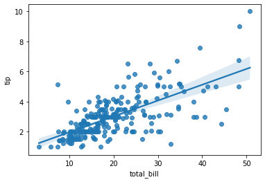
# %%
# ci = 신뢰구간 지정. confidence Interval -> 모집단 분포 추정
sns.regplot(x='total_bill', y='tip', data=tips, ci=99);