1. 머신러닝과 딥러닝의 차이
미프 2차를 통해, 머신러닝과 딥러닝을 실습해보았다.
x주제에 대한 df을 받아서, 데이터 전처리를 거치고, 머신러닝과 딥러닝을 각각 돌려보면서 더 우수한 성능을 나타내는지 비교분석했다.
신기하게도, 머신러닝 모델에서 더 좋은 mae와 mape 값을 얻을 수 있었다.
이를 통해, 알 수 있는 사실은 다음과 같다.
- 데이터 전처리가 가능하며, df와 같이 정형 데이터를 다룰 때는 머신러닝이 더 좋다.
- 이미지, 텍스트, 음성 데이터와 같이 비정형 데이터를 다룰 때는 딥러닝이 더 좋다.
2. CNN
- 이미지 데이터를 사용하여 딥러닝하는 방법이다.
- 전에 했던 딥러닝은 Functional API를 사용하는 방법이지만, CNN의 경우에는 Sequential API 방식을 사용한다.
- suquential API은 Convolutional Layer를 사용한다.
- Convolutional은 1. Conv2D /// 2. Maxpool2D를 사용한다.
- Conv2D는 1) filters 2) kernel_size, 3) strides, 4) padding, 5) activation를 매개변수로 사용한다.
- Maxpool2D는 1) pool_size, 2) strides를 매개변수로 사용한다.
-
1) 원래 하던 functional 방식을 사용하기 전에, 전처리를 한다고 생각하면 된다.
-
2) functional은 flatten을 사용하는 것처럼, 2차원으로 만들어서 쫙 핀 다음, 학습을 하기 때문에, 위치 정보의 소실이 발생한다.
-
3) sequential은 convolutional layer를 거쳐서 위치 정보가 보존된 서로 다른 feature을 갖는 feature map을 만든다.
-
333) filters는 depth/hidden layer와 유사하다. 값 설정은 우리가 hidden layer 값 정한는 것과 같이 우리가 정한다.
-
4) Conv2D 방법은 kernel_size가 strides 보폭만큼 이동하면서 kernel 크기에서 random 값이 들어있는 컴퓨터가 생성한 filter map와의 연산을 통해 새로운 값을 도출하고 activation을 거친 다음에, 해당 값을 새로운 map에 입력하며, feaure map의 크기는 작아진다.
-
4-1) 필요에 따라, padding을 할 수 있다. padding은 이전 feautre map의 size를 유지시킨다.
-
5) Maxpool 방법은 pool_size가 stride 보폭만큼 이동하는데 pool_size에서 가장 큰 값을 도출하고 해당 값을 갖는 map을 형성하며 크기가 작아진다.
-
5-1) 보통 pool_size와 stride는 같은 값을 갖는다.
- 이미지 데이터의 x_train shape을 보면 (60000, 28, 28)을 나타내는 경우, 그냥 사용했었지만 흑백(1) or 색의 이미지 데이터(3)의 경우 (60000, 28, 28, 1(흑백), 3(색))의 shape을 사용해야 한다.
- 이미지 데이터의 y_train의 경우 원래 (60000,)였는데, (60000, 10)과 같이 원핫인코딩을 통해서 1차원에서 2차원으로 바꿔줘야한다.
- 주의할 점이 하나 있는데, class_n이 100과 같이 너무 크다면,
- 원핫인코딩을 하지 않고 model.compile(loss = 'sparse_categorical_crossentropy')로 두는 것이 더 좋다.
- 4차원의 데이터에 대해서 MinMax 스케일링을 하게 된다면, 기존에 알던 방식이 아닌 공식을 사용해서 작성해야 한다.
- 원핫인코딩의 경우, 어떤 관측치에 대해서 할지 모른다. 그래서 get_dummies가 아닌 to_categorical 라이브러리를 사용해야 한다.
- MinMax 스케일링

# x_train으로 fit해준다.
max_n = x_train.max()
min_n = x_train.min()

x_train = (x_train - max_n) / (max_n - min_n)
x_test = (x_test - max_n) / (max_n - min_n)
=======================================================
- 원핫인코딩
from tf.keras.utils import to_categorical       # 만약에 안된다면 keras.utils import to_categorical 해보셈

class_n = len(np.unique(y_train))

y_train = to_categorical(y_train, class_n)
y_test = to_categorical(y_test, class_n)

x_train.shape, y_train.shape
<출력>
((14979, 28, 28, 1), (14979, 10))
2-1. MinMax scaling 방법 2가지
-
standard scaling의 경우는 train = (train-mean)/std의 식이다.
-
xtrain.shape을 보면 (40000,28,28,3)이 출력된다면 (,,,3)을 통해서 색 이미지임을 알 수 있다.
-
색은 R,G,B를 통해서 표현된다.
-
그래서 스케일링 방법이 2가지가 존재한다.
- RGB를 한번에 스케일
- R/G/B 따로 스케일을 진행하고 합치기(np.stack)
- 1번 방법
해당 방법은 위에서 정리했다.

- 2번 방법

# min, max fit
tr_r_max, tr_r_min = train_x[:,:,:,0].max(), train_x[:,:,:,0].min()
tr_g_max, tr_g_min = train_x[:,:,:,1].max(), train_x[:,:,:,1].min()
tr_b_max, tr_b_min = train_x[:,:,:,2].max(), train_x[:,:,:,2].min()

# train_x
train_r_mm = (train_x[:,:,:,0] - tr_r_min) / (tr_r_max - tr_r_min)
train_g_mm = (train_x[:,:,:,1] - tr_g_min) / (tr_g_max - tr_g_min)
train_b_mm = (train_x[:,:,:,2] - tr_b_min) / (tr_b_max - tr_b_min)

# test_x
test_r_mm = (test_x[:,:,:,0] - tr_r_min) / (tr_r_max - tr_r_min)
test_g_mm = (test_x[:,:,:,1] - tr_g_min) / (tr_g_max - tr_g_min)
test_b_mm = (test_x[:,:,:,2] - tr_b_min) / (tr_b_max - tr_b_min)

# R/G/B 분할된거 하나로 합치기
train_x_mm = np.stack((train_r_mm, train_g_mm, train_b_mm), axis=3)

# shape, (max 값) 확인
train_x_mm.shape

<출력>
(40000, 32, 32, 3)
3. Functional API 예제
-----------------------------------------------------------
# 1. 세션 클리어 : 메모리에 기존 모델 구조가 남아있으면 정리해줘.
keras.backend.clear_session()

-----------------------------------------------------------
# 2. 레이어 사슬처럼 엮기
il = tf.keras.layers.Input(shape=[28, 28, 1])     # x_train shape임
h = tf.keras.layers.Flatten()(il)

h = tf.keras.layers.Dense(256, activation='relu')(h)
h = tf.keras.layers.Dense(256, activation='relu')(h)
h = tf.keras.layers.BatchNormalization()(h)
h = tf.keras.layers.Dropout(0.2)(h)

h = tf.keras.layers.Dense(128, activation='relu')(h)
h = tf.keras.layers.Dense(128, activation='relu')(h)
h = tf.keras.layers.BatchNormalization()(h)
h = tf.keras.layers.Dropout(0.2)(h)

h = tf.keras.layers.Dense(64, activation='relu')(h)
h = tf.keras.layers.Dense(64, activation='relu')(h)
h = keras.layers.BatchNormalization()(h)
h = tf.keras.layers.Dropout(0.2)(h)

ol = tf.keras.layers.Dense(10, activation='softmax')(h)
-----------------------------------------------------------

# 3. 모델의 시작과 끝 지정
model = tf.keras.models.Model(il, ol)
-----------------------------------------------------------
# 4. 컴파일
model.compile(optimizer='adam',
              loss = 'categorical_crossentropy',
              metrics='accuracy')

model.summary()
-----------------------------------------------------------------------
# 5. Early stop
from tf.keras.callbacks import EarlyStopping

es = EarlyStopping(es = EarlyStopping(monitor='val_loss',
                  min_delta=0,
                  patience=5,
                  verbose = 1,         # 어느 epoch에서 얼리스토핑이 적용되었는지 보여줌
                  restore_best_weights=True,)
----------------------------------------------------------------------------
# 6. model 학습
model.fit(x_train, y_train,
          epochs=100000,
          verbose=1,
          validation_split=0.2,
          callbacks=[es],)           # callbacks에 여러개 쓸 수 있어서 [es]로 넣어준거래

----------------------------------------------------------------------------
3-1. model 평가
-
평가 방법은 1. evaluate 2. accuracy / classification_report 있다.
-
원핫 인코딩 한 것을 다시 묶어주는 코드 argmax
-
평가 지표 및 실제 데이터 확인을 위해 필요
# 7. model 평가
model.evaluate(x_test, y_test)

<출력>
118/118 [==============================] - 0s 2ms/step - loss: 0.3140 - accuracy: 0.9076
[0.3139810562133789, 0.9076101183891296]
----------------------------------------------------------------------------

# 7-1 model 평가
y_pred = model.predict(x_test)

y_pred_arg = np.argmax(y_pred, axis = 1)
test_y_arg = np.argmax(y_test, axis = 1)

from sklearn.metrics import accuracy_score, classification_report

# 1
accuracy_score(test_y_arg, y_pred_arg)

# 2
print(classification_report(test_y_arg, y_pred_arg))

<출력>
0.9076101468624833

              precision    recall  f1-score   support

           0       0.93      0.89      0.91       357
           1       0.85      0.91      0.88       365
           2       0.93      0.94      0.93       374
           3       0.93      0.91      0.92       392
           4       0.97      0.85      0.91       406
           5       0.95      0.96      0.96       377
           6       0.86      0.92      0.89       372
           7       0.89      0.93      0.91       374
           8       0.86      0.86      0.86       385
           9       0.91      0.94      0.92       343

    accuracy                           0.91      3745
   macro avg       0.91      0.91      0.91      3745
weighted avg       0.91      0.91      0.91      3745
3-2. 시각화
3-2-1. 실제 데이터 확인
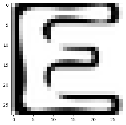
letters_str = "ABCDEFGHIJ"

rand_idx = np.random.randint(0, len(y_pred_arg))
test_idx = test_y_arg[rand_idx]
pred_idx = y_pred_arg[rand_idx]
class_prob = np.floor( y_pred[rand_idx]*100 )

print(f'idx = {rand_idx}')
print(f'해당 인덱스의 이미지는 {letters_str[test_idx]}')
print(f'모델의 예측 : {letters_str[pred_idx]}')
print(f'모델의 클래스별 확률 : ')
print('-------------------')
for idx, val in enumerate(letters_str) :
    print(val, class_prob[idx])
print('=================================================')

if test_y_arg[rand_idx] == y_pred_arg[rand_idx] :
    print('정답')
else :
    print('땡')

plt.imshow(x_test[rand_idx], cmap='Greys')
plt.show()

<출력>
idx = 2016
해당 인덱스의 이미지는 E
모델의 예측 : E
모델의 클래스별 확률 :
-------------------
A 4.0
B 15.0
C 2.0
D 0.0
E 69.0
F 0.0
G 4.0
H 0.0
I 1.0
J 0.0
=================================================
3-2-2. 틀린 이미지 확인
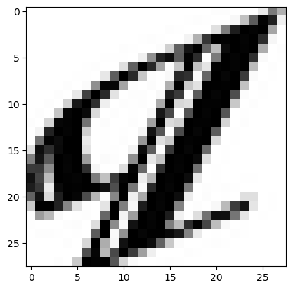
# 1
temp = (test_y_arg == y_pred_arg)
false_idx = np.where(temp==False)[0]
false_len = len(false_idx)
false_len

# 2
letters_str = "ABCDEFGHIJ"

rand_idx = false_idx[np.random.randint(0, false_len)]
test_idx = test_y_arg[rand_idx]
pred_idx = y_pred_arg[rand_idx]
class_prob = np.floor( y_pred[rand_idx]*100 )

print(f'idx = {rand_idx}')
print(f'해당 인덱스의 이미지는 {letters_str[test_idx]}')
print(f'모델의 예측 : {letters_str[pred_idx]}')
print(f'모델의 클래스별 확률 : ')
print('-------------------')
for idx, val in enumerate(letters_str) :
    print(val, class_prob[idx])
print('=================================================')

if test_y_arg[rand_idx] == y_pred_arg[rand_idx] :
    print('정답')
else :
    print('땡')

plt.imshow(x_test[rand_idx], cmap='Greys')
plt.show()
<출력>
idx = 1359
해당 인덱스의 이미지는 I
모델의 예측 : C
모델의 클래스별 확률 :
-------------------
A 1.0
B 0.0
C 30.0
D 2.0
E 6.0
F 9.0
G 27.0
H 6.0
I 5.0
J 8.0
================================================
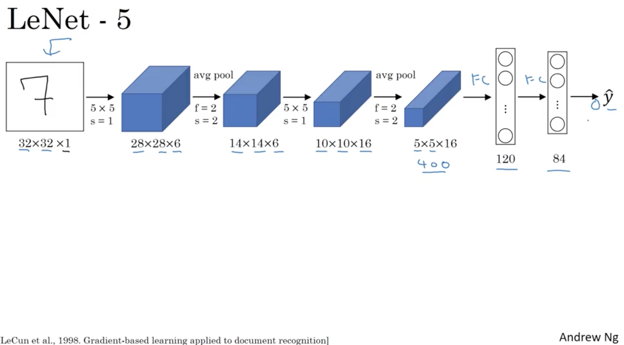
4. convolutional layer
- 1) 32 x 32 x 1의 input layer를 받는다.
- 2) filters은 안나왔지만 우리가 원하는 값으로 설정한다.
- 2-1) kernal_size인 filter의 크기는 5x5이고 strides=1임으로 한칸 씩 이동하면서 값을 연산하고 저장한다.
- 2-2) 32에서 28로 줄어든것으로 보아 padding은 없고, 32x1에서 28x6이 된것으로 보아 filters는 6임을 알 수 있다.
- 3) pool이 진행됐으며, pool_size는 2이고 2칸씩 이동한다. 2칸의 값중 큰값만 14개가 저장된다. filters의 크기는 변하지 않는다.
- 4) kernal_size는 5이고 1칸씩 이동하면서 값을 저장한다. 계산해보면 5에서 출발해서 1칸씩이니까 14-5+1 = 10의 크기를 갖는 map이 만들어진다.
- 4-1) 14 x 6에서 10 x 16이 된것으로 보아 filters는 16임을 알 수 있다.
- 5) pool의 크기는 2이고 2칸씩이동하니까 10의 절반인 5의 크기를 갖는 map이 만들어지고 filterts는 변하지 않는다.
- 6) 만약 padding이 있다면, 이전 feature map의 사이즈가 유지된다.
- 000) 400개의 픽셀을 이제 flatten 시킨다음 hidden layer를 두고 out layer(y_train의 shape만큼)를 받는다.
5. Sequential API 예제 1.
- 데이터 분할됐다고 가정.

# 1. x-reshape

x_train.shape

<출력>
(60000, 28, 28)

_, r, w = x_train.shape
x_train = x_train.reshape(x_train.reshape[0], r, w, -1)
x_test = x_test.reshape(x_test.reshape[0], r, w, -1)
* -1은 앞에 3개에 데이터를 넣고 4번째에 남은 데이터 넣겠다 의미임.
* 여기서는 1이랑 같음

x_train.shape, x_test.shape

<출력>
((60000, 28, 28, 1), (10000, 28, 28, 1))
-----------------------------------------------------------

# 2. Min-Max scaling

max_n, min_n = x_train.max(), x_train.min()

x_train = (x_train - min_n) / (max_n - min_n)
x_test = (x_test - min_n) / (max_n - min_n)

x_train.max(), x_train.min()

<출력>
(1.0, 0.0)
-----------------------------------------------------------

# 3. 원핫인코딩

from tensorflow.keras.utils import to_categorical

class_n = len(np.unique(y_train))

y_train = to_categorical(y_train, class_n)
y_test = to_categorical(y_test, class_n)

y_train.shape

<출력>
(60000, 10)
-----------------------------------------------------------

# 4. Sequential API 작성

- 1) 라이브러리 불러오기
import tensorflow as tf
from tensorflow import keras

from tensorflow.keras.backend import clear_session
from tensorflow.keras.models import Model, Sequential
from tensorflow.keras.layers import Input, Dense, Conv2D, MaxPool2D, Flatten, BatchNormalization, Dropout


- 2) Sequential API

## Sequential API

# 1번. 세션 클리어
keras.backend.clear_session()

# 2번. 레이어 조립
il = Input(shape=(28,28,1))

h = Conv2D(filters=128,              # Conv2D를 통해 제작하려는 Feature map의 수
        kernel_size=(3,3),       # filter의 가로세로 size
        strides=(1,1),           # convolutional filter의 이동 보폭
        padding='same',          # filter가 훑기 전에 상하좌우로 픽셀을 덧붙임
        activation='relu')(il)     # activation 주의!!!

h = Conv2D(filters=128,              # Conv2D를 통해 제작하려는 Feature map의 수
        kernel_size=(3,3),       # filter의 가로세로 size
        strides=(1,1),           # convolutional filter의 이동 보폭
        padding='same',          # filter가 훑기 전에 상하좌우로 픽셀을 덧붙임
        activation='relu')(h)    # activation 주의!!!

h = MaxPool2D(pool_size=(2,2),      # pooling filter의 가로세로 사이즈
            strides=(2,2))(h)      # pooling filter의 이동보폭

h = Flatten()(h)
h = Dense(128, activation='relu')(h)
ol = Dense(10, activation='softmax')(h)

# 3번. 모델 컴파일
model = Model(il, ol)
model.compile(loss = 'categorical_crossentropy', metrics='accuracy', optimizer = 'adam')

model.summary()

<출력>
_________________________________________________________________
 Layer (type)                Output Shape              Param #
=================================================================
 input_1 (InputLayer)        [(None, 28, 28, 1)]       0      >
                                                            >
 conv2d (Conv2D)             (None, 28, 28, 128)       1280     >
                                                            >
 conv2d_1 (Conv2D)           (None, 28, 28, 128)       147584  >
                                                            >
 max_pooling2d (MaxPooling2  (None, 14, 14, 128)       0        >
 D)                                                              >
                                                            >
 flatten (Flatten)           (None, 25088)             0         >
                                                           >
 dense (Dense)               (None, 128)               3211392
                                                          >
 dense_1 (Dense)             (None, 10)                1290      >
                                                            >
=================================================================
Total params: 3361546 (12.82 MB)
Trainable params: 3361546 (12.82 MB)
Non-trainable params: 0 (0.00 Byte)
_________________________________________________________________
# 5. Early stopping

from keras.callbacks import EarlyStopping

es = EarlyStopping(monitor='val_loss',
                   min_delta=0,
                   patience=5,
                   verbose=1,
                   restore_best_weights=True)

model.fit(x_train, y_train, epoches = 100, verbose = 1,
	      validation_size=0.2, callbacks = [es])
-----------------------------------------------------------

# 6. model 평가

- 1번 평가
model.evaluate(x_test, y_test)

- 2번 평가
y_pred = model.predict(test_x)

y_pred_arg = np.argmax(y_pred, axis =1)
test_y_arg = np.argmax(test_y, axis = 1)

accuracy_score(test_y_arg, y_pred_arg)
print( classification_report(test_y_arg, y_pred_arg)
-----------------------------------------------------------