📊 RNN(Recurrent Neural Network)

📌 RNN이란?

• 정의
  - 히든 노드가 엣지로 연결되어 순환구조를 이루는(directed cycle) 인공신경망의 한 종류이다.
  - 타임스탭(time step)을 사용하여 이전 epoch의 출력값을 다음 epoch의 입력값에 추가하여 사용한다.
  
  
• 활성화 함수
  - tanh
  
  
• 특징
  - 학습 시간과 길이가 길어질수록 초기 입력값의 형태를 잊어버린다.
  → [ LSTM or GRU 층을 사용하여 초기 입력값의 형태를 지속적으로 회고한다. ]
  
  
• 활용
  - 텍스트 분류, 품사 태깅, 문서 요약, 문서 작성, 기계번역, 이미지 캡션 등

📊 RNN 실습

📌 RNN 실습

1. 라이브러리 Import

import numpy as np
import matplotlib.pyplot as plt
from keras.models import Sequential
from keras.layers import LSTM, GRU, Dense
from keras.optimizers import Adam
from keras.callbacks import EarlyStopping

---

2. 데이터 준비

x = np.array([[1,2,3], [2,3,4], [3,4,5], [4,5,6], [5,6,7], [10,11,12], [20,30,40], [30,40,50]])
y = np.array([4, 5, 6, 7, 8, 13, 50, 60])
print(x.shape)
print(y.shape)
# (8, 3)
# (8,)

---

3. RNN층 입력에 맞게 feature reshaping

x = x.reshape(x.shape[0], x.shape[1], 1)
print(x.shape)
# (8, 3, 1)

---

4. RNN 모델 구축

model = Sequential()
model.add(LSTM(units=10, input_shape=(3, 1), activation='tanh'))
model.add(Dense(units=5, activation='relu'))
model.add(Dense(units=1, activation='linear'))

print(model.summary())
# Model: "sequential"
# _________________________________________________________________
#  Layer (type)                Output Shape              Param #   
# =================================================================
#  lstm (LSTM)                 (None, 10)                480       
#
#  dense (Dense)               (None, 5)                 55        
#
#  dense_1 (Dense)             (None, 1)                 6         
#
# =================================================================
# Total params: 541
# Trainable params: 541
# Non-trainable params: 0
# _________________________________________________________________
# None

---

5. 모델 학습 최적화 설정

model.compile(optimizer=Adam(learning_rate=0.001), loss='mse', metrics=['mae'])

---

6. 모델 학습

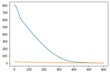
es = EarlyStopping(
    monitor='loss',
    patience=10
)

history = model.fit(
    x=x,
    y=y,
    batch_size=1,
    epochs=1000,
    verbose=0,
    callbacks=[es]
)
plt.plot(history.history['loss'], label='loss')
plt.plot(history.history['mae'], label='mae')

---

7. 모델 예측값, 실제값 비교

pred = model.predict(x)
print('예측값 : ', pred.flatten())
print('실제값 : ', y)
# 예측값 :  [ 4.0216813  4.9978     6.031329   7.012912   7.975519  12.964263  50.64533   58.025978 ]
# 실제값 :  [ 4  5  6  7  8 13 50 60]