import numpy as np
import pandas as pd
import seaborn as sns
import matplotlib.pyplot as plt
import seaborn as sns
from sklearn.preprocessing import StandardScaler, PolynomialFeatures
from sklearn.linear_model import LinearRegression, Ridge, Lasso
import warnings
warnings.filterwarnings(action='ignore')
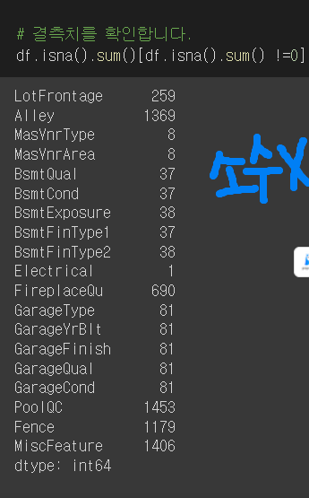
#결측치 확인
df.isna().sum()[df.isna().sum() !=0]/len(df)
- [] len(df)를 나눠주는 이유는 ..?
# 고유한 값이 너무 많은 컬럼도 예측에 도움이 되지 않으니 확인하고 삭제해주겠습니다.
df.nunique()[df.nunique()/len(df)>0.7]
cols = ['Id', 'LotArea']
df.drop(cols, axis=1, inplace=True)
#타겟분포확인
# 왼쪽으로 치우쳐진 분포입니다. 주택 판매 가격이 400000을 넘지 않는 샘플만 다시 추출하도록 하겠습니다.
df = df[df['SalePrice']<400000]
sns.histplot(df['SalePrice'], bins=50)
# 수치형 컬럼과 타겟간의 상관관계를 확인해보겠습니다. 상관관계가 높은 상위 10개 컬럼만 보도록하겠습니다.
# target = SalePrice
df.corr()['SalePrice'].sort_values(ascending=False).head(11)
Modeling
from sklearn.model_selection import train_test_split
X = df.drop('SalePrice', axis=1)
y = df['SalePrice']
X_train, X_test, y_train, y_test = train_test_split(X, y, test_size=0.2, random_state=42)
모델링에 필요한 두 가지 전처리
- Scaling scaler = StandardScaler()
- Encoding
# 결측치를 먼저 평균으로 모두 채워주겠습니다.
X_trian.fillna(X_train.mean(), inplace=True)
X_test.fillna(X_test.mean(), inplace=True)
#수치형 변수만 스케일링
#dtype으로 수치형 변수 판별하기
numeric_feats = X_train.dtypes[X_train.dtypes != "object"].index
scaler = StandardScaler()
X_train[numeric_feats] = scaler.fit_transform(X_train[numeric_feats])
X_test[numeric_feats] = scaler.transform(X_test[numeric_feats])
# .T가 행과 열 위치 바꿈
X_train[numeric_feats].describe().T[['mean','std']]
One-Hot encoding
from category_encoders import OneHotEncoder
ohe = OneHotEncoder()

X_train_ohe = ohe.fit_transform(X_train)
X_test_ohe = ohe.fit_transform(X_test)
(X_train_ohe.dtypes == 'object').sum()
mszoning_cols = [x for x in X_train_ohe.columns if 'MSZoning' in x]
X_train_ohe[mszoning_cols].head(3)

#범주형 특성이 어떻게 변환이 되었는지 확인
ohe.category_mapping
기준모델 : 평균이용
from sklearn.metrics import r2_score, mean_absolute_error

baseline = [y_train.mean()]*len(y_train)
baseline_r2 = r2_score(y_train, baseline)
baseline_mae = mean_absolute_error(y_train, baseline)
다중선형회귀 OLS
def print_score(model, X_train, y_train, X_test, y_test) :
    train_score = np.round(model.score(X_train, y_train) , 3)
    val_score = np.round(np.mean(cross_val_score(model, X_train, y_train, scoring='r2', cv=3).round(3)),3)
    test_score = np.round(model.score(X_test, y_test),3)

    return train_score, val_score, test_score
from sklearn.model_selection import cross_val_score

# 선형회귀를 ols라는 객체에 저장합니다.
ols = LinearRegression()

# 모델 학습
ols.fit(X_train_ohe, y_train)

# 성능 비교
ols_train, ols_val, ols_test = print_score(ols,X_train_ohe, y_train, X_test_ohe, y_test)
ridge regression 모델 만들기
for alpha in [0.01, 0.1, 1.0, 1, 100.0, 1000.0, 10000.0]:
	print(f"Ridge Regression, alpha={alpha}")

    #모델학습
    ridge = Ridge(alpha=alpha)
    ridge.fit(X_train_ohe, y_train)

    #성능확인()#print_score 위에서 만들었던 함수
    print_score(ridge,X_train_ohe, y_train, X_test_ohe, y_test)

    #coefficients 계수
    #절대값 상위 40개의 회귀계수만 불러오기
    coefficients = pd.Series(ridge.coef_, X_train_ohe.columns)
    idx = np.abs(coefficients).head(40).index
sklearn에서 내장된 교차검증 알고리즘 ridgeCV
