이 글은 아래 영상을 참고하여 재구성하였습니다.
https://youtu.be/AA621UofTUA
NLP 논문의 역사
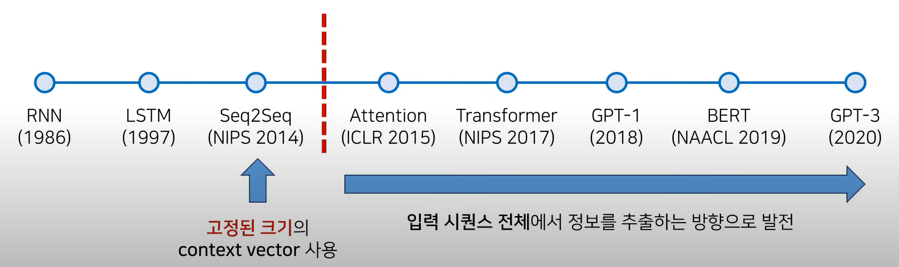
- Seq2Seq의 성능적인 한계
- Transformer로 비약적인 성능 향상 이룩 → 이후 Attention 기법을 많이 사용하게 됨
- Attention 이후에는 입력 sequence 전체에서 정보를 추출하는 방향으로 발전
Seq2Seq 한계점
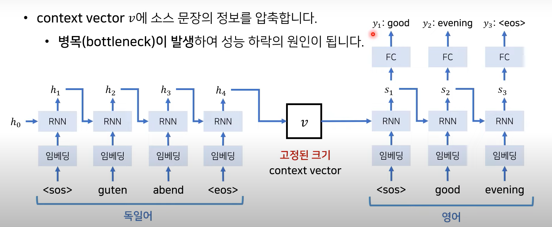
<sos> : start of sequence
<eos> : end of sequence
- context vector v에 소스 문장의 정보를 압축하는데, 병목현상의 원인이 됨
(context vector는 고정된 크기니까 압축에 한계가 있음) → vector가 체함. 성능 저하됨.
→ 그럼 고정된 값으로 받지말고 매번 소스 문장에서의 출력 전부를 입력으로 받으면 어떨까?
Attention
연속성 개념을 배제하고 단어들의 상관관계를 구하는데 집증
데이터가 충분히 많으면 모델이 알아서 성능을 뽑아내는 게 대세
Seq2Seq + Attention
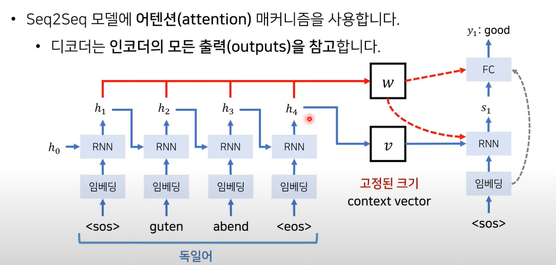
출력 단어가 생성될 때 마다 w값(Attention) 반영
Causality Masking
transformer는 모든 단어를 병렬적으로 처리하기 때문에 autoregressive 한 특성이 없음
→ 목표하는 문장의 일부를 가려서 인위적으로 연속성을 학습하게 함 → Causality Masking
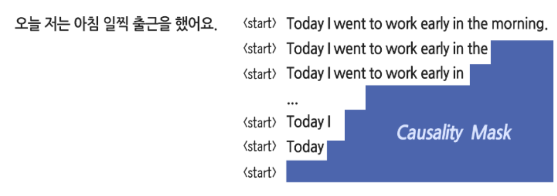
→ Autoregressive 하게 문장 생성
-
code
좌측은 실제 마스크의 형태, 우측은 마스킹이 적용된 Attention입니다. 마스킹은 마스킹 할 영역을 -∞로 채우고 그 외 영역을 0으로 채운 배열을 Dot-Product된 값에 더해주는 방식으로 진행됩니다. 후에 진행될 Softmax는 큰 값에 높은 확률을 할당하는 함수이므로 -∞로 가득 찬 마스킹 영역에는 무조건 0의 확률을 할당하게 됩니다.
import numpy as np
import tensorflow as tf
import matplotlib.pyplot as plt

def make_dot_product_tensor(shape):
    A = tf.random.uniform(shape, minval=-3, maxval=3)
    B = tf.transpose(tf.random.uniform(shape, minval=-3, maxval=3), [1, 0])

    return tf.tensordot(A, B, axes=1)

def generate_causality_mask(seq_len):
    mask = 1 - np.cumsum(np.eye(seq_len, seq_len), 0)
    return mask

sample_tensor = make_dot_product_tensor((20, 512))
sample_tensor = sample_tensor / tf.sqrt(512.)

mask = generate_causality_mask(sample_tensor.shape[0])

fig = plt.figure(figsize=(7, 7))

ax1 = fig.add_subplot(121)
ax2 = fig.add_subplot(122)

ax1.set_title('1) Causality Mask')
ax2.set_title('2) Masked Attention')

ax1.imshow((tf.ones(sample_tensor.shape) + mask).numpy(), cmap='cividis')

mask *= -1e9
ax2.imshow(tf.nn.softmax(sample_tensor + mask, axis=-1).numpy(), cmap='cividis')

plt.show()
Basic Architecture
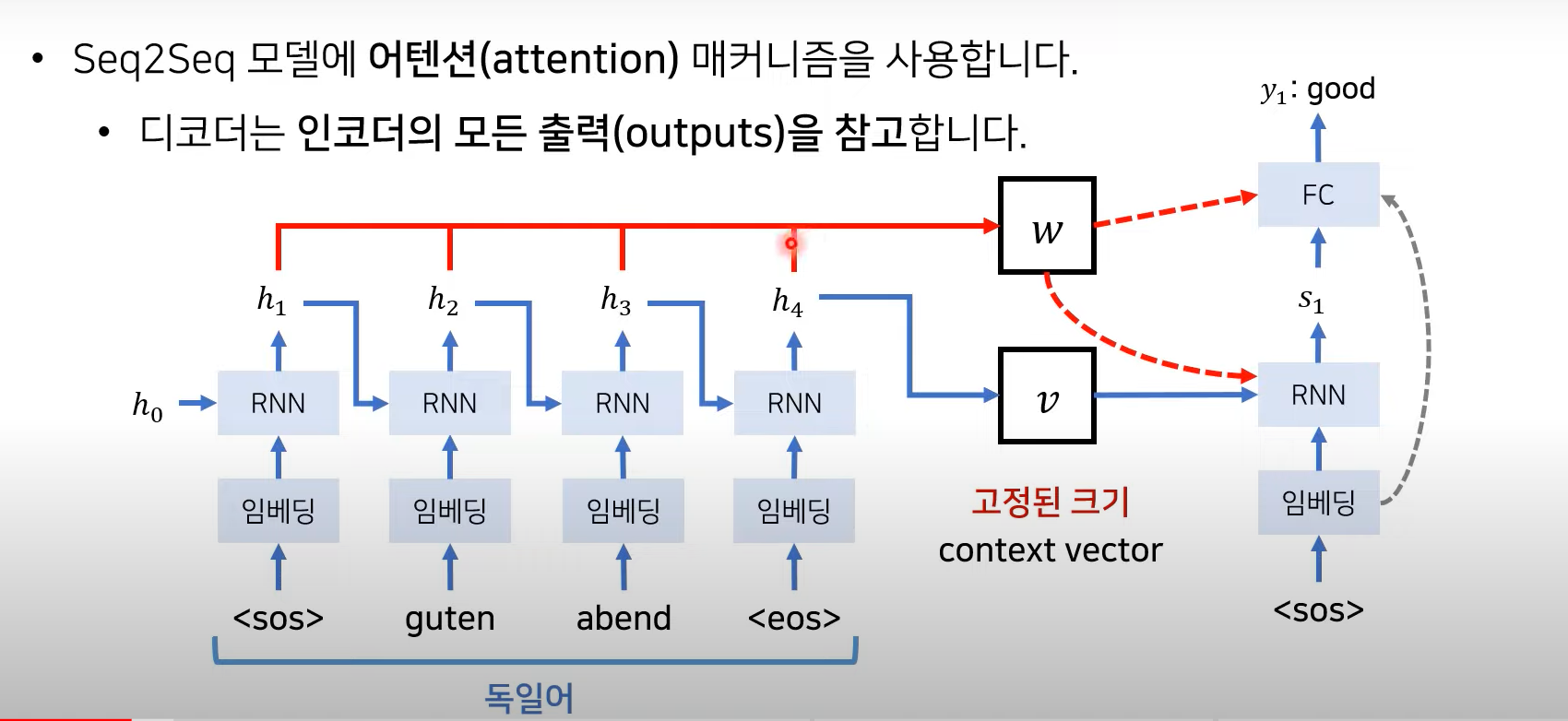
= source 문장의 각 단어의 hidden state 값
= output의 hidden state 값
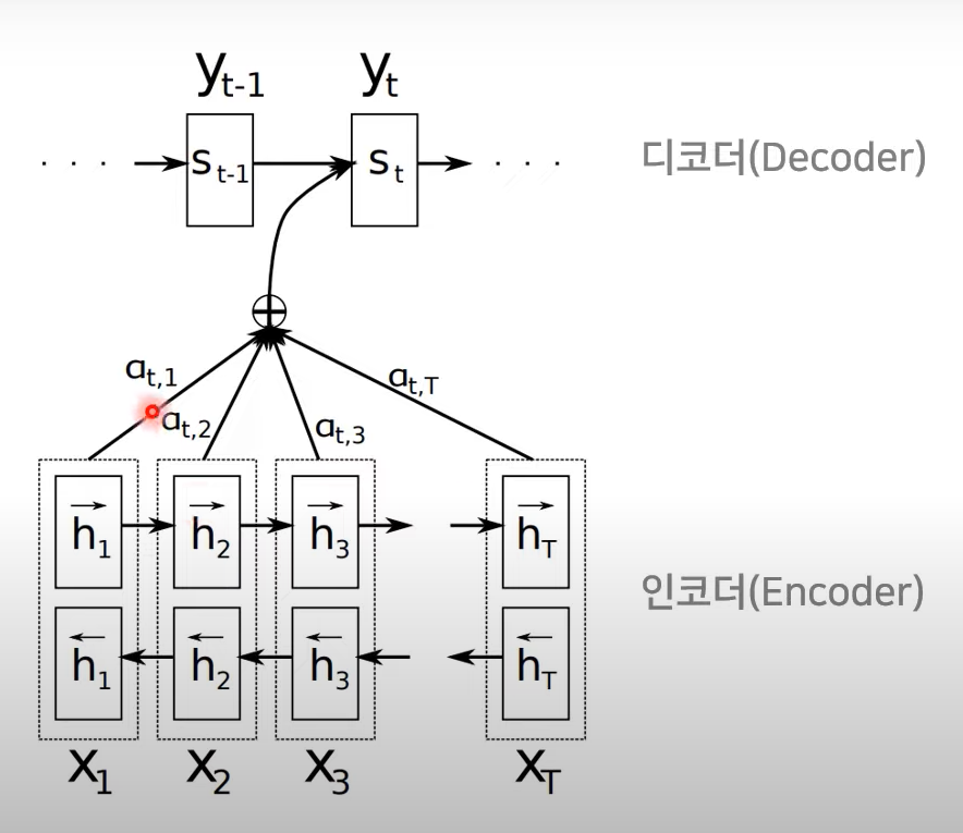
- source 문장의 output h1 h2 h3 h4 를 모두 참고하겠다 → weighted sum 이 network에 적용
- h1, h2, h3, h4 값에 각각 얼마나 많은 가중치를 두어서 vector에 곱할 것인가? → Attention
Decoder
- 인코더의 출력 정보 중 어떤 정보가 중요한지 계산!
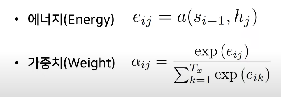
Energy
= 현재의 디코더가 처리(단어를 생성) 중인 인덱스
= 각각의 인코더 출력 인덱스
: 모든 출력값 고려하는 의미
: 이전(i-1)에 출력했던 단어가 만들어냈던(decoding 과정에서) hidden state
: encoder part의 각각의 hidden state
Weight
1) k=1 부터 j 까지 각각의 encoder에서 출력된
2) i-1번째 hidden state로부터 만들어진
3) 그로부터 만들어지는 에너지
Softmax function 계산에 의해 해당 에너지에 대한 가중치
이렇게 계산된 가중치 와 를 곱하여 합계를 구함(weighted sum)
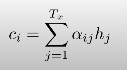
weighted sum = context vector
→ 각각 단어별로 가중치가 계산이 되며, 이는 hidden state에 곱해짐
context vector() 의 형태로 에 반영되어
decoder로부터 단어 생성!
어텐션 시각화도 가능
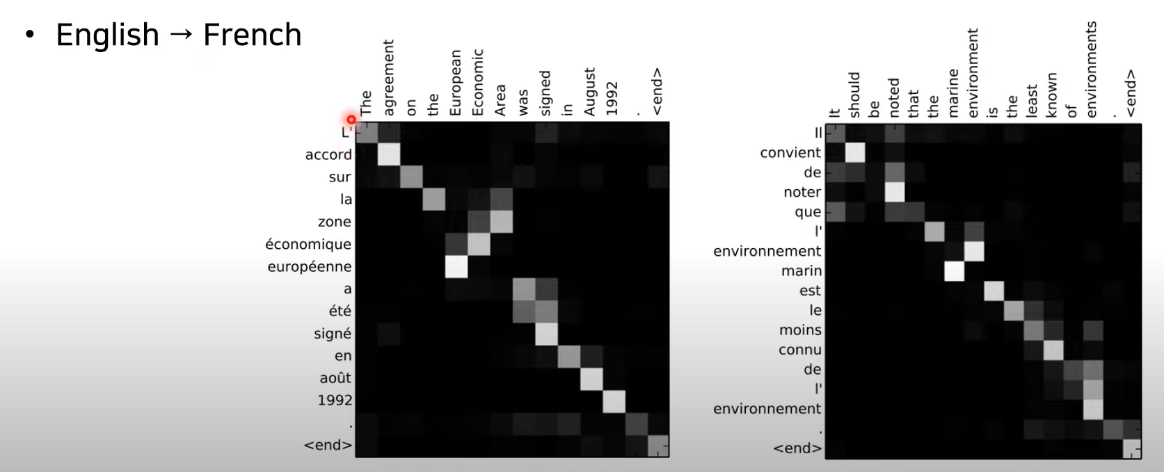
Transformer Model Architecture
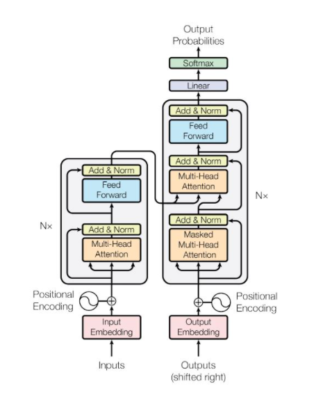
왼쪽이 encoder, 오른쪽이 decoder
- 모델에 RNN과 CNN 이 없음 → 단어 순서에 관한 정보가 없다. → Positional encoding으로 해결
- Encoder와 decoder로 구성되며, Attention 과정을 여러 레이어에서 반복
순서
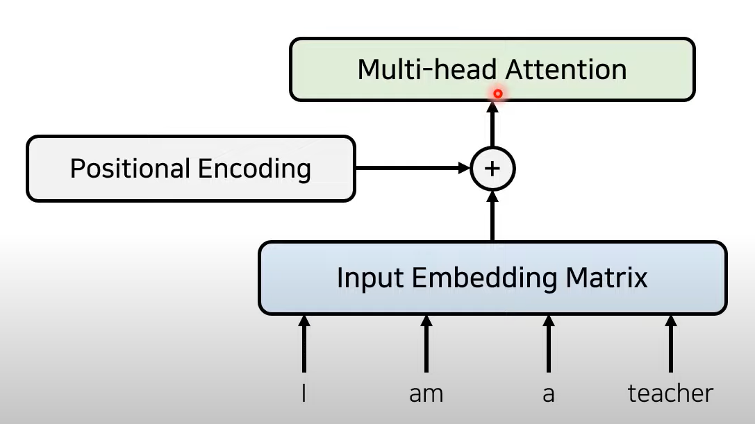
Embedding → (Multihead) Attention → Positional encoding
1) embedding
- embedding_dim 설정(일반적으로 512)
I am a teacher (4단어) → 4*512 shape의 vector가 생성된다.
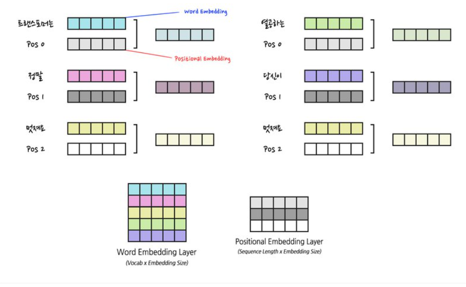
2) Positional encoding
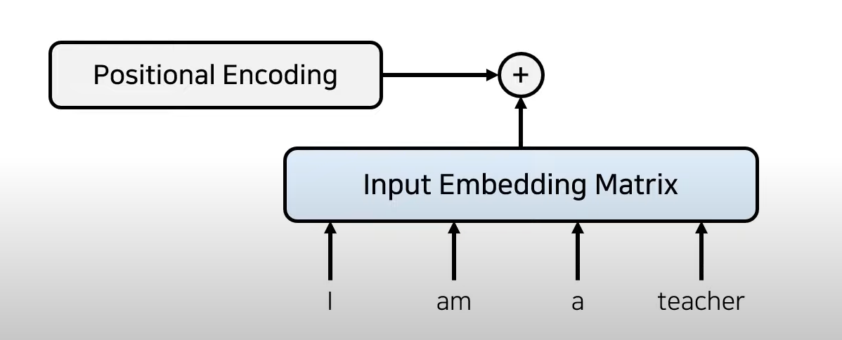
위치에 대한 정보가 담긴 별도의 encoding 정보를 Embedding matrix에 더함(element-wise sum)
-
Positional encoding의 조건
1) 각 Time-step마다 고유의 Encoding 값을 출력해야 한다.
2) 서로 다른 Time-step이라도 같은 거리라면 차이가 일정해야 한다.
3) 순서를 나타내는 값이 특정 범위 내에서 일반화가 가능해야 한다.
4) 같은 위치라면 언제든 같은 값을 출력해야 한다.
-
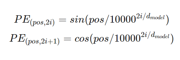
sin과 cosine이용한 positinal encoding(position은 각각 고유하다)
-
code
import numpy as np

def positional_encoding(pos, d_model):
    def cal_angle(position, i):
        return position / np.power(10000, int(i) / d_model)

    def get_posi_angle_vec(position):
        return [cal_angle(position, i) for i in range(d_model)]

    sinusoid_table = np.array([get_posi_angle_vec(pos_i) for pos_i in range(pos)])

    sinusoid_table[:, 0::2] = np.sin(sinusoid_table[:, 0::2])
    sinusoid_table[:, 1::2] = np.cos(sinusoid_table[:, 1::2])

    return sinusoid_table

pos = 7
d_model = 4
i = 0

print("Positional Encoding 값:\n", positional_encoding(pos, d_model))

print("")
print("if pos == 0, i == 0: ", np.sin(0 / np.power(10000, 2 * i / d_model)))
print("if pos == 1, i == 0: ", np.sin(1 / np.power(10000, 2 * i / d_model)))
print("if pos == 2, i == 0: ", np.sin(2 / np.power(10000, 2 * i / d_model)))
print("if pos == 3, i == 0: ", np.sin(3 / np.power(10000, 2 * i / d_model)))

print("")
print("if pos == 0, i == 1: ", np.cos(0 / np.power(10000, 2 * i + 1 / d_model)))
print("if pos == 1, i == 1: ", np.cos(1 / np.power(10000, 2 * i + 1 / d_model)))
print("if pos == 2, i == 1: ", np.cos(2 / np.power(10000, 2 * i + 1 / d_model)))
print("if pos == 3, i == 1: ", np.cos(3 / np.power(10000, 2 * i + 1 / d_model)))
2)-1 Positional Embedding
→ 이후 BERT 모델에 적용되는 개념
3) Multi-head Attention
-
등장배경(직관 이해해보기)
바나나라는 단어가 512차원의 Embedding을 가진다고 가정합시다. 그중 64차원은 노란색에 대한 정보를 표현하고, 다른 64차원은 달콤한 맛에 대한 정보를 표현할 겁니다. 같은 맥락으로 바나나의 형태, 가격, 유통기한까지 모두 표현될 수 있겠죠. 저자들은 '이 모든 정보들을 섞어서 처리하지 말고, 여러 개의 Head로 나누어 처리하면 Embedding의 다양한 정보를 캐치할 수 있지 않을까?' 라는 아이디어를 제시합니다.
Positional encoding으로부터의 위치 정보가 담긴 Attention을 Multihead attention 이라고 함
- Decoder 에서의 Attention은, 각각의 단어가 서로에게 어떤 연관성을 가지고 있는지를 구하기 위해 사용 → 전반적인 입력 문장 (I, am, a, teacher) 각각이 어떤 단어와 유사한지 알고 문맥에 대한 정보를 학습함!
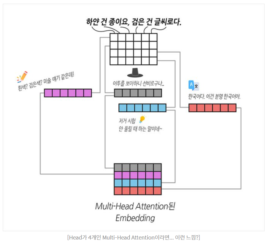
- 주로 8개를 사용
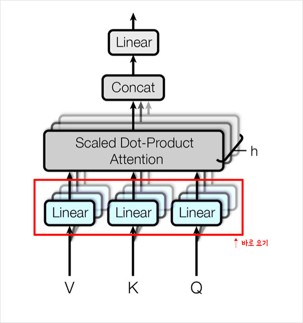
- Head로 쪼갠 Embedding들끼리 유사한 특성을 가진다는 보장이 없기 때문에 앞단에 Linear 레이어를 추가
- linear layer는 Multi-Head Attention이 잘 동작할 수 있는 적합한 공간으로 Embedding을 매핑
4) Position-wised Feed forward network
Attention is all you need paper 뽀개기
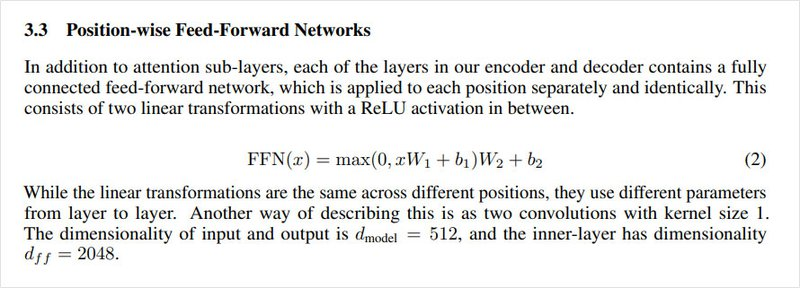
: linear layer
: Relu
- 예를 들면 10단어로 이루어진 Attention된 문장
[10, 512]를[10, 2048]공간으로 매핑, 활성함수를 적용한 후 다시[10, 512]공간으로 되돌리는 것 - Position-wise FFN
- Linear layer는 convolutional layer의 역할
5) Layer Normalization
- Feature 차원에서 정규화하는 방법 ex) 10단어의 Embedding된 문장을 예로 [10, 512]에서 512차원 Feature를 정규화하여 분포를 일정하게 맞춰주는 것
- Batch Normalization은 정규화를 Batch 차원에서 진행하는 것이고 Layer Normalization은 정규화를 Feature 차원에서 진행하는 것이다.
Introduction to Deep Learning Normalization
6) Residual learning
- layer가 깊어질수록 생기는 문제 네트워크가 깊어질 수록 Optimize(Train)하는 것이 어렵기 때문에, 얕은 네트워크가 더 좋은 성능을 보이게 된다.
- 수식
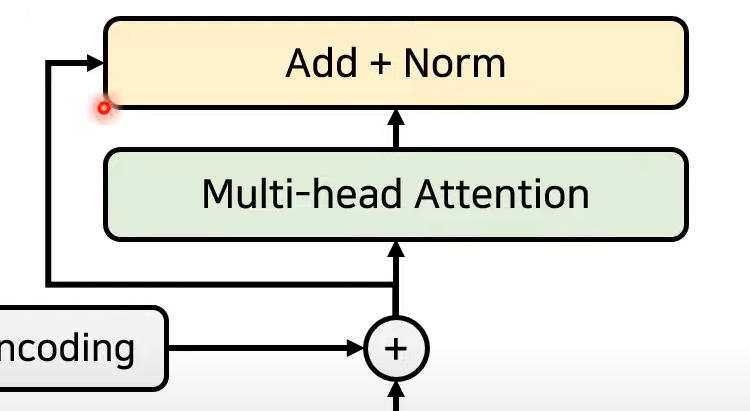
- Resnet에서 이용되는, 특정 layer를 건너뛰어서 학습하는 기법
- 기존 정보를 입력받으면서 추가적으로 잔여된 부분만 학습(add)
- 이후 Normalization
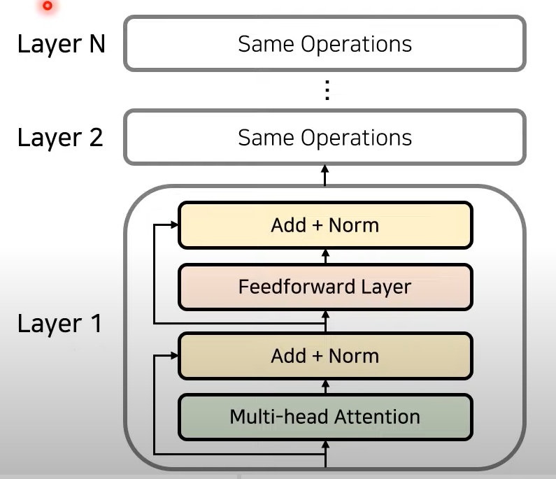
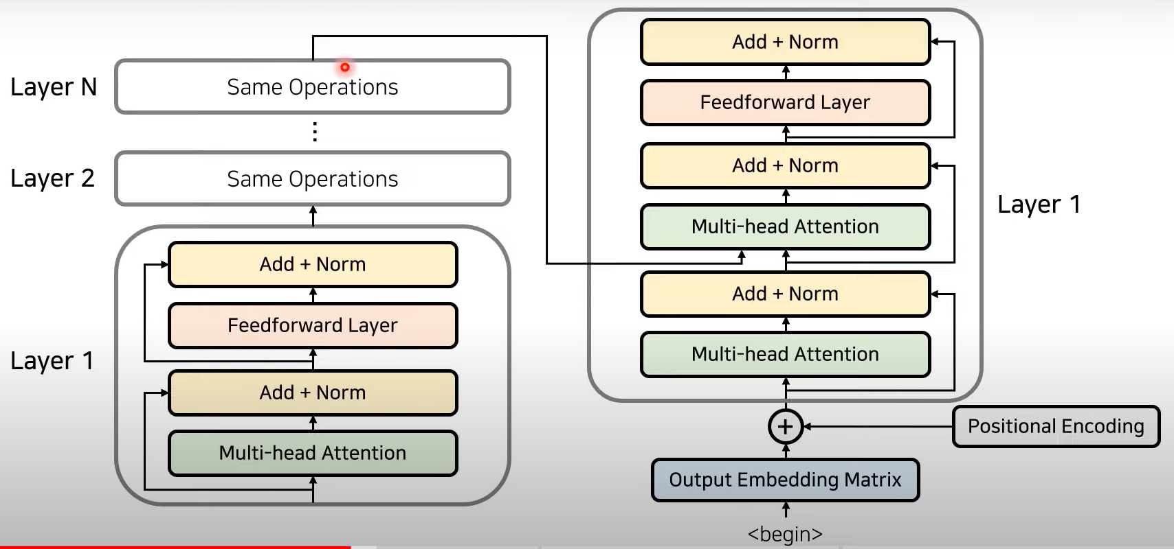
- Attention과 Normalization 반복하는 방식으로 Layer 중첩
- Same Operation
7) Learning rate schedular
- Learning Rate를 수식에 따라 변화시키며 사용

위 수식을 따르게 되면 까지는 가 선형적으로 증가 하고, 이후에는 에 비례해 점차 감소하는 모양새 를 보이게 됩니다.
→ 초반 학습 효율 증가, 후반에 디테일한 튜닝
- code
import matplotlib.pyplot as plt
import numpy as np

d_model = 512
warmup_steps = 4000

lrates = []
for step_num in range(1, 50000):
    lrate = (np.power(d_model, -0.5)) * np.min(
        [np.power(step_num, -0.5), step_num * np.power(warmup_steps, -1.5)])
    lrates.append(lrate)

plt.figure(figsize=(6, 3))
plt.plot(lrates)
plt.show()
8) Weight sharing
- 하나의 Weight를 두 개 이상의 레이어가 동시에 사용
- 트랜스포머에서는 Decoder의 Embedding 레이어와 출력층 Linear 레이어의 Weight를 공유하는 방식을 사용
- 튜닝해야 할 파라미터 수가 감소하기 때문에 학습에 더 유리하며 자체적으로 Regularization 되는 효과
Encoder to Decoder
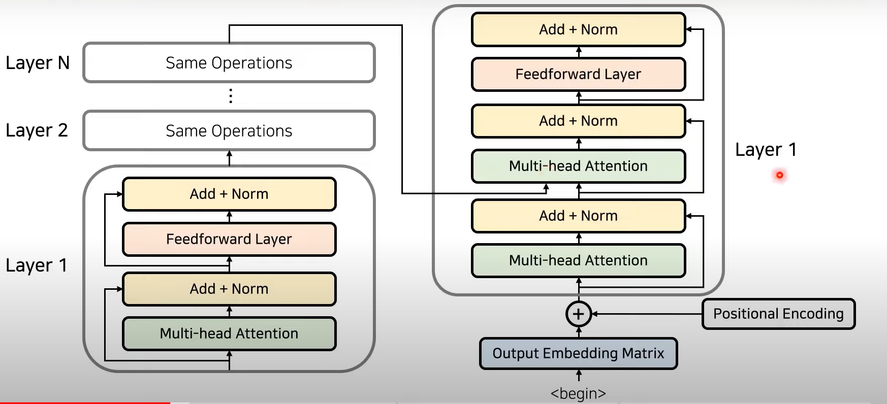
- Encoder의 마지막 Layer의 output이 decoder의 layer에 들어감!
→ Decoder의 각각의 출력 정보가 Encoder로부터 의 출력을 받아 사용할 수 있도록 만듦
Decoder
- decoder 또한 각 단어 정보를 받아서 encoding값을 추가한 뒤에 입력을 넣게 됨
- decoder에서는 두개의 Layer를 사용함
ex) 'I am a teacher→ 나는 선생님이다'로 번역 시
i am a teacher는 encoder의 input
'나는 선생님이다' 는 decoder의 input
encoder의 마지막 layer로부터의 output을 정보로 받는다
→ decoder의 '선생님' 이라는 단어가 input (i am a teacher)에서 어떤 단어와 가장 큰 연관성을 가지는 지 정보를 받아 알 수 있는 것!(여기서는 teacher 곘지)
layer 관점에서의 구조
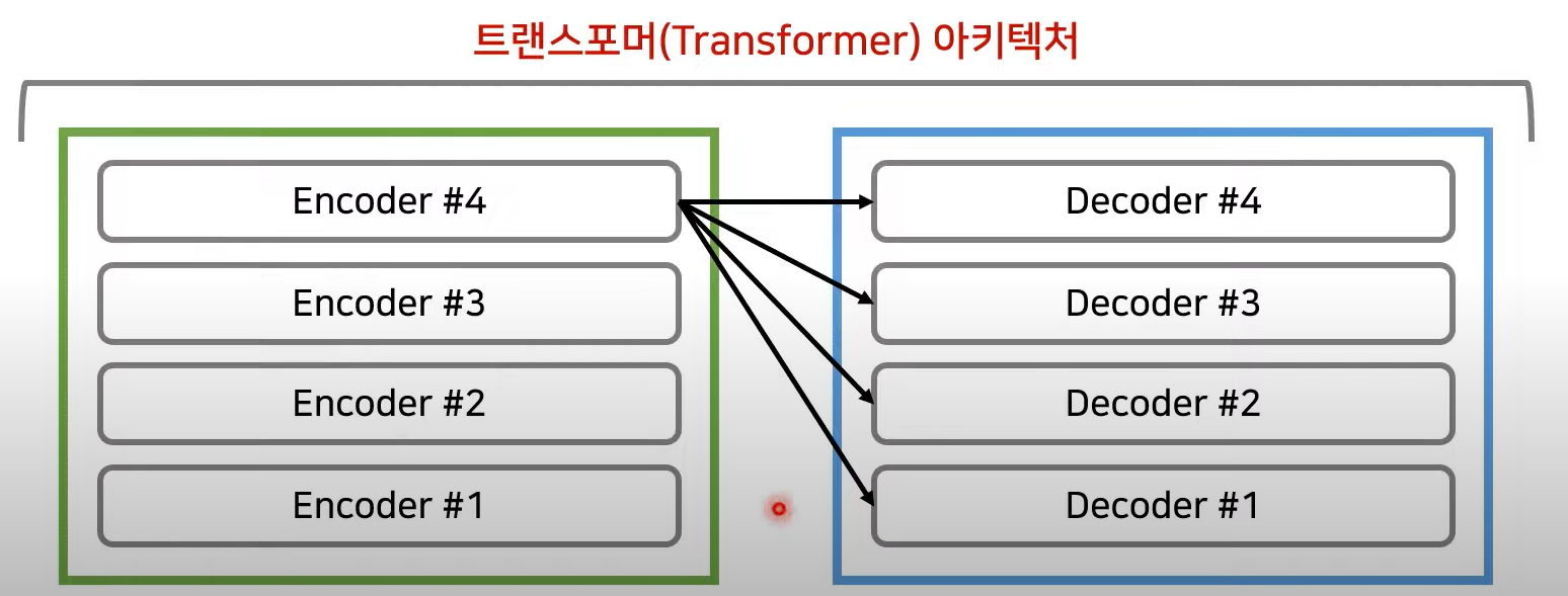
Transformer에서, 보통 Encoder와 Decoder는 같은 수의 layer를 갖고 있음!
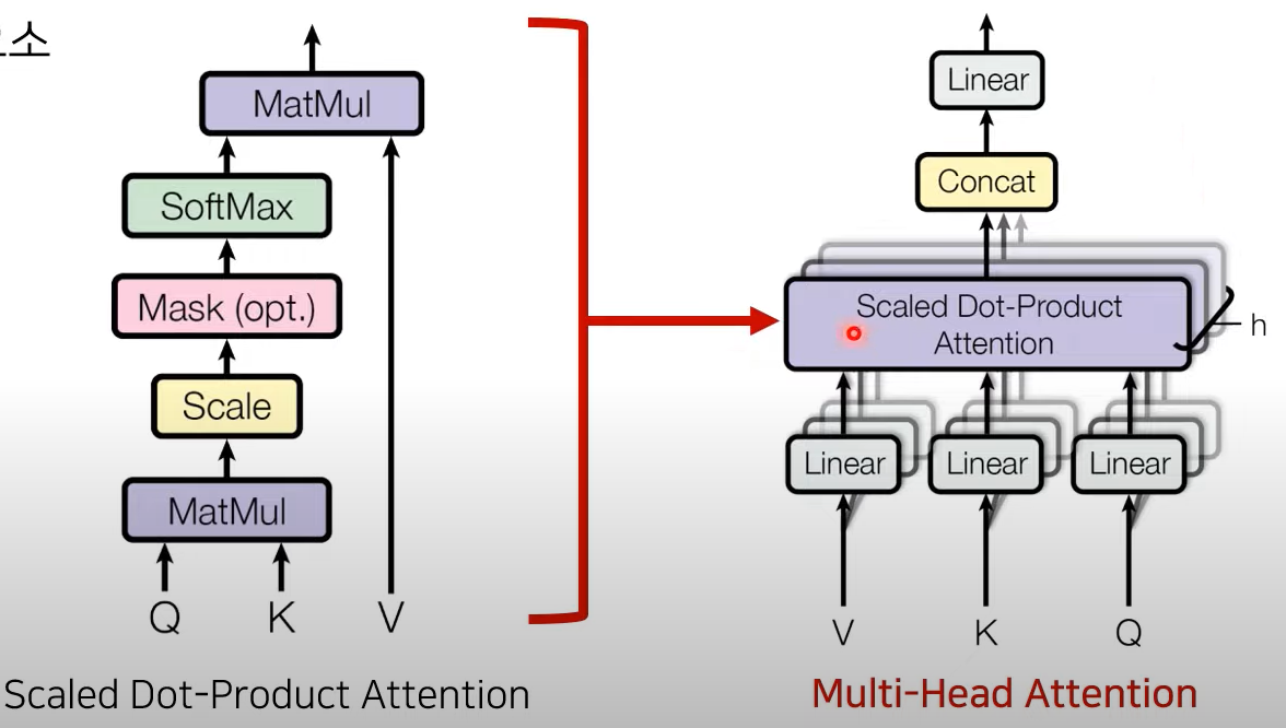
Q,K,V : Attention을 위한 세 가지 입력 요소
어떠한 단어가 다른 단어와 어떠한 연관성을 지니는가?
- Query : 무언가를 물어보는 주체
- Key : 물어보는 대상
- Value는 value
예시
I am a teacher → 에서 self attention을 진행하고 싶을 때,
I 라는 단어가 다른 단어와 어떠한 연관성이 있는지 알고 싶어서 내부의 다른 단어들에 물어본다!
I : query
I am a teacher : Key
각각의 key 에 대해서 attention score를 구할 수 있음
이후에,(왼쪽 그림 참고)
Q K 가 각각 input으로 들어가서 Matmul → Scaling → mask 씌워줌 → Softmax 취함 → 확률값 return
결과적으로 어떤 단어와 가장 높은 연관성을 지니는 지 알 수 있음!
확률값과 value값을 위해서 가중치가 적용된 attention value를 구할 수 있음!
(오른쪽 그림 참고)
각 V,K,Q 는 h개의 서로 다른 V, K,Q로 구분됨
Attention의 입력값과 출력값의 dimension은 같아야 하기 때문에, head로부터의 attention 값들의 concat을 수행해서 일자로 붙이고 마지막 linear layer를 붙여서 output을 내보내게 됨
구조에서 Q, K, V 보기
encoder 파트에서 Key, Value
decoder의 Multihead Attention에서는 Query
Multihead Attention Equation
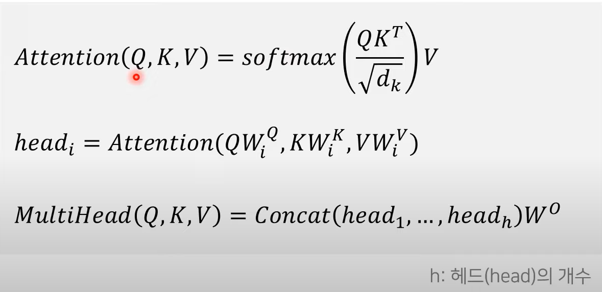
Q 와 K의 유사도를 dot product 로 계산하여 를 attention 가중치로 삼음
하는 이유 ! : Embedding 차원 수가 깊어지면 깊어질수록 Dot-Product의 값은 커지게 되어 Softmax를 거치고 나면 미분 값이 작아지는 현상이 나타난다. 그 경우를 대비해 Scale 작업이 필요하다.
-
code
import tensorflow as tf
import matplotlib.pyplot as plt

def make_dot_product_tensor(shape):
    A = tf.random.uniform(shape, minval=-3, maxval=3)
    B = tf.transpose(tf.random.uniform(shape, minval=-3, maxval=3), [1, 0])

    return tf.tensordot(A, B, axes=1)

length = 30
big_dim = 1024.
small_dim = 10.

big_tensor = make_dot_product_tensor((length, int(big_dim)))
scaled_big_tensor = big_tensor / tf.sqrt(big_dim)
small_tensor = make_dot_product_tensor((length, int(small_dim)))
scaled_small_tensor = small_tensor / tf.sqrt(small_dim)

fig = plt.figure(figsize=(13, 6))

ax1 = fig.add_subplot(141)
ax2 = fig.add_subplot(142)
ax3 = fig.add_subplot(143)
ax4 = fig.add_subplot(144)

ax1.set_title('1) Big Tensor')
ax2.set_title('2) Big Tensor(Scaled)')
ax3.set_title('3) Small Tensor')
ax4.set_title('4) Small Tensor(Scaled)')

ax1.imshow(tf.nn.softmax(big_tensor, axis=-1).numpy(), cmap='cividis')
ax2.imshow(tf.nn.softmax(scaled_big_tensor, axis=-1).numpy(), cmap='cividis')
ax3.imshow(tf.nn.softmax(small_tensor, axis=-1).numpy(), cmap='cividis')
ax4.imshow(tf.nn.softmax(scaled_small_tensor, axis=-1).numpy(), cmap='cividis')

plt.show()