[딥러닝 논문 리뷰] 1.AlexNet

박범규·2022년 1월 21일

AlexNet CNN 논문리뷰 딥러닝

딥러닝 논문 리뷰

목록 보기

2/3

*공부 및 복습 용도의 글입니다. 부족하거나 틀린 부분이 있다면 댓글로 알려주신다면 감사드리겠습니다.

2022/02/14 수정 - bias initializing에 문제가 있었음.

AlexNet

AlexNet은 Alex Krizhevsky, Ilya Sutskever와 Geoffrey Hinton이 설계한 CNN architecture로, 2012년 ILSVRC에서 큰 격차로 우승하여 이름을 알렸다. AlexNet을 설명한 논문 ImageNet Classification with Deep Convolutional Neural Networks를 살펴보자.

Architecture

ReLU Non-Linearity

Activation function으로 Sigmoid나 tanh를 주로 사용하던 기존 모델과 달리 AlexNet에서는 ReLU를 사용했다.
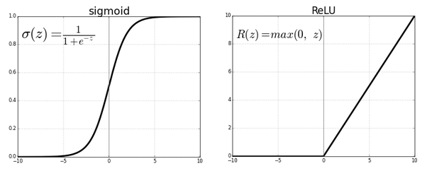
ReLU는 x값이 양수일 경우 기울기가 일정하기 때문에 gradient vanishing 현상이 일어나지 않고, 연산 비용이 비교적 적다. 실제로 CIFAR-10을 가지고 비교한 결과 25% training error rate에 도달하는 시간이 6배 가량 빠르다고 한다.

Training on Multiple GPUs

더 큰 네트워크를 위해 2개의 GPU로 병렬 연산을 수행했다. 두 GPU는 3번째 convolutional layer와 FC(Fully connected) layer를 제외하면 독립적으로 훈련을 진행했다.
GPU를 하나만 썼을 경우와 비교하여, training error를 1~2% 가량 줄였고 시간도 약간 더 빨랐다고 한다.

Local Response Normalization

ReLU는 sigmoid형 함수와는 달리 input normalization이 필수는 아니다. 하지만 AlexNet에서는 local response normalization를 적용해 오차를 약 1~2% 줄였다고 한다.
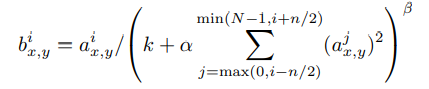
식이 조금 복잡해 보이지만, 간단히 말해 주변 kernel에 비해 큰 값이 나온 곳을 정규화하는 것이다. i번째 kernel map의 x, y 지점의 값을 (i-n/2)번째~(i+n/2)번째 kernel map의 x, y 지점의 값들을 더해 나누게 된다.
최근에는 잘 쓰이지 않는 방법이라고 한다.

Overlapping Pooling

전통적으로 pooling은 pooling unit의 크기와 stride의 크기가 같아 마치 격자와 같이 나뉜다. 하지만 AlexNet에서는 pooling unit의 크기가 더 큰 overlapping pooling 기법을 사용해 약 0.4%의 오차 감소를 얻었다.
정확한 이유는 나오지 않으나, overlapping pooling을 적용했을 시 과적합 현상이 조금 해소된다고 한다.

Reducing Overfitting

Data Augmentation

과적합을 방지하는 가장 쉬운 방법 중 하나는 label-preserving transformation(라벨 보존 변형)을 사용하여 데이터셋을 늘리는 것이다.
논문에서는 두 가지 방법의 변형을 사용하는데, 그 중 첫 번째는 반전과 crop이다. 원본 256 X 256의 이미지를 랜덤하게 잘라 224 X 224 이미지를 만들고, 전체를 또다시 반전시킨 버전을 만들면 데이터셋이 2048배로 늘어난다. (* 224 X 224는 논문의 오타이고, stride와 padding을 따져봤을 때 227이 정확한 값이라고 한다.)
두 번째 방법은 PCA(주성분분석)를 통해 RGB 값을 변형하는 것이다.
논문에 따르면 이러한 data augmentation 없이는 심각한 과적합에 시달린다고 한다.

Dropout

Dropout은 히든 레이어의 특정 뉴런의 출력을 일정 확률로 0으로 만드는 것을 말한다. 이는 뉴런들의 co-adaption을 줄인다. 즉 불확실성을 부여해 특정 뉴런에 의존하지 못하도록 하는 것이다.
이 방법 또한 과적합을 크게 줄여주었다.

Details of Learning

찾아보니 loss function은 cross entropy를 사용했다고 한다. Multi-class classification에는 거의 대부분 cross entropy를 사용한다고.
Weight decay를 사용하였다. weight 파라미터에 크기가 너무 커지지 않게 페널티를 주는 방법으로, 보통 L2 regularization을 많이 사용한다.
각 weight는 $\mu=0,\sigma=0.01$ 의 정규분포로 초기화했고, bias는 2, 4, 5번째 convolutional layer와 FC layer들에 한해 1로 초기화했다. 이는 양수값을 줘서 ReLU의 초기 학습을 가속시키기 위해서이다.
learning rate는 우선 모든 층을 똑같이 맞춘 후, 오차가 더이상 줄지 않을때 10으로 나누는 식으로 조정했다. 초기 learning rate 0.01로 시작해 학습이 끝날 때까지 세 번 나뉘었다.
120만 장의 이미지를 약 90번씩 학습시켜 6일이 걸렸다.

Results

2010년도 ILSVRC 데이터로 돌려본 결과, top-1과 top-5 부문에서 각각 오차율 37.5%와 17.0%를 기록했다. 당년도 우승 모델은 47.1%, 28.2%였고 이를 크게 뛰어넘은 수치이다.
2012년도 ILSVRC에도 참가하여, top-5 부문 오차율을 16.4%까지 줄일 수 있었다.

코드 구현

Papers with Code에 올라온 이 코드와 twinjui님의 코드를 참고하여 작성하였다.

import numpy as np
import pandas as pd
import tensorflow as tf

# define model parameters
NUM_EPOCHS = 1000
NUM_CLASSES = 10
IMAGE_SIZE = 227
BATCH_SIZE = 16

데이터 전처리. twinjui님의 코드를 사용했다.

from tensorflow.keras.utils import to_categorical
from sklearn.model_selection import train_test_split
from tensorflow.keras.datasets import cifar10

def zero_one_scaler(image):
    return image/255.0

def get_preprocessed_ohe(images, labels, pre_func=None):
    # preprocessing 함수가 입력되면 이를 이용하여 image array를 scaling 적용.
    if pre_func is not None:
        images = pre_func(images)
    # OHE 적용    
    oh_labels = to_categorical(labels)
    return images, oh_labels

# 학습/검증/테스트 데이터 세트에 전처리 및 OHE 적용한 뒤 반환 
def get_train_valid_test_set(train_images, train_labels, test_images, test_labels, valid_size=0.15, random_state=2021):
    # 학습 및 테스트 데이터 세트를  0 ~ 1사이값 float32로 변경 및 OHE 적용. 
    train_images, train_oh_labels = get_preprocessed_ohe(train_images, train_labels)
    test_images, test_oh_labels = get_preprocessed_ohe(test_images, test_labels)
    
    # 학습 데이터를 검증 데이터 세트로 다시 분리
    tr_images, val_images, tr_oh_labels, val_oh_labels = train_test_split(train_images, train_oh_labels, test_size=valid_size, random_state=random_state)
    
    return (tr_images, tr_oh_labels), (val_images, val_oh_labels), (test_images, test_oh_labels )

# CIFAR10 데이터 재 로딩 및 Scaling/OHE 전처리 적용하여 학습/검증/데이터 세트 생성. 
(train_images, train_labels), (test_images, test_labels) = cifar10.load_data()
print(train_images.shape, train_labels.shape, test_images.shape, test_labels.shape)
(train_images, train_labels), (val_images, val_labels), (test_images, test_labels) = \
    get_train_valid_test_set(train_images, train_labels, test_images, test_labels, valid_size=0.2, random_state=2021)

print(train_images.shape, train_labels.shape, val_images.shape, val_labels.shape, test_images.shape, test_labels.shape)

from tensorflow.keras.utils import Sequence
import cv2
import sklearn

# 입력 인자 images_array labels는 모두 numpy array로 들어옴. 
# 인자로 입력되는 images_array는 전체 32x32 image array임. 
class CIFAR_Dataset(Sequence):
    def __init__(self, images_array, labels, batch_size=BATCH_SIZE, augmentor=None, shuffle=False, pre_func=None):
        '''
        파라미터 설명
        images_array: 원본 32x32 만큼의 image 배열값. 
        labels: 해당 image의 label들
        batch_size: __getitem__(self, index) 호출 시 마다 가져올 데이터 batch 건수
        augmentor: albumentations 객체
        shuffle: 학습 데이터의 경우 epoch 종료시마다 데이터를 섞을지 여부
        '''
        # 객체 생성 인자로 들어온 값을 객체 내부 변수로 할당. 
        # 인자로 입력되는 images_array는 전체 32x32 image array임.
        self.images_array = images_array
        self.labels = labels
        self.batch_size = batch_size
        self.augmentor = augmentor
        self.pre_func = pre_func
        # train data의 경우 
        self.shuffle = shuffle
        if self.shuffle:
            # 객체 생성시에 한번 데이터를 섞음. 
            #self.on_epoch_end()
            pass
    
    # Sequence를 상속받은 Dataset은 batch_size 단위로 입력된 데이터를 처리함. 
    # __len__()은 전체 데이터 건수가 주어졌을 때 batch_size단위로 몇번 데이터를 반환하는지 나타남
    def __len__(self):
        # batch_size단위로 데이터를 몇번 가져와야하는지 계산하기 위해 전체 데이터 건수를 batch_size로 나누되, 정수로 정확히 나눠지지 않을 경우 1회를 더한다. 
        return int(np.ceil(len(self.labels) / self.batch_size))
    
    # batch_size 단위로 image_array, label_array 데이터를 가져와서 변환한 뒤 다시 반환함
    # 인자로 몇번째 batch 인지를 나타내는 index를 입력하면 해당 순서에 해당하는 batch_size 만큼의 데이타를 가공하여 반환
    # batch_size 갯수만큼 변환된 image_array와 label_array 반환. 
    def __getitem__(self, index):
        # index는 몇번째 batch인지를 나타냄. 
        # batch_size만큼 순차적으로 데이터를 가져오려면 array에서 index*self.batch_size:(index+1)*self.batch_size 만큼의 연속 데이터를 가져오면 됨
        # 32x32 image array를 self.batch_size만큼 가져옴. 
        images_fetch = self.images_array[index*self.batch_size:(index+1)*self.batch_size]
        if self.labels is not None:
            label_batch = self.labels[index*self.batch_size:(index+1)*self.batch_size]
        
        # 만일 객체 생성 인자로 albumentation으로 만든 augmentor가 주어진다면 아래와 같이 augmentor를 이용하여 image 변환
        # albumentations은 개별 image만 변환할 수 있으므로 batch_size만큼 할당된 image_name_batch를 한 건씩 iteration하면서 변환 수행. 
        # 변환된 image 배열값을 담을 image_batch 선언. image_batch 배열은 float32 로 설정. 
        image_batch = np.zeros((images_fetch.shape[0], IMAGE_SIZE, IMAGE_SIZE, 3), dtype='float32')
        
        # batch_size에 담긴 건수만큼 iteration 하면서 opencv image load -> image augmentation 변환(augmentor가 not None일 경우)-> image_batch에 담음. 
        for image_index in range(images_fetch.shape[0]):
            #image = cv2.cvtColor(cv2.imread(image_name_batch[image_index]), cv2.COLOR_BGR2RGB)
            # 원본 image를 IMAGE_SIZE x IMAGE_SIZE 크기로 변환
            image = cv2.resize(images_fetch[image_index], (IMAGE_SIZE, IMAGE_SIZE))
            # 만약 augmentor가 주어졌다면 이를 적용. 
            if self.augmentor is not None:
                image = self.augmentor(image=image)['image']
                
            # 만약 scaling 함수가 입력되었다면 이를 적용하여 scaling 수행. 
            if self.pre_func is not None:
                image = self.pre_func(image)
            
            # image_batch에 순차적으로 변환된 image를 담음.               
            image_batch[image_index] = image
        
        return image_batch, label_batch
    
    # epoch가 한번 수행이 완료 될 때마다 모델의 fit()에서 호출됨. 
    def on_epoch_end(self):
        if(self.shuffle):
            #print('epoch end')
            # 원본 image배열과 label를 쌍을 맞춰서 섞어준다. scikt learn의 utils.shuffle에서 해당 기능 제공
            self.images_array, self.labels = sklearn.utils.shuffle(self.images_array, self.labels)
        else:
            pass
            
def zero_one_scaler(image):
    return image/255.0

train_ds = CIFAR_Dataset(train_images, train_labels, batch_size=BATCH_SIZE, augmentor=None, shuffle=True, pre_func=zero_one_scaler)
val_ds = CIFAR_Dataset(val_images, val_labels, batch_size=BATCH_SIZE, augmentor=None, shuffle=False, pre_func=zero_one_scaler)

가져온 데이터를 시각화해 확인

from matplotlib import pyplot
from keras.datasets import cifar10
# summarize loaded dataset
print('Train: X=%s, y=%s' % (train_ds[0][0][0].shape, train_ds[0][1][0].shape))
print('Test: X=%s, y=%s' % (val_ds[0][0][0].shape, val_ds[0][1][0].shape))
# plot first few images
for i in range(9):
    # define subplot
    pyplot.subplot(330+1+i)
    # plot raw pixel data
    pyplot.imshow(train_ds[0][0][i])
# show the figure
pyplot.show()

AlexNet 정의.

from tensorflow.keras.layers import *

class AlexNet(tf.keras.Model):
    def __init__(self, num_classes=NUM_CLASSES):
        super().__init__()
#         self.weight = tf.keras.initializers.RandomNormal(mean=0., stddev=1.)
#         self.bias = tf.keras.initializers.Constant(1.)
        self.lrn = lambda x: tf.nn.local_response_normalization(x, depth_radius=5, alpha=0.0001, beta=0.75, bias=2)
        self.regularizer = tf.keras.regularizers.l2(l2=0.0005)
        self.net = tf.keras.Sequential([
            Conv2D(
                filters=96, 
                kernel_size=11, 
                strides=4, 
#                 kernel_initializer=self.weight, 
                kernel_regularizer=self.regularizer
            ),
            ReLU(),
            Lambda(self.lrn),
            MaxPool2D(pool_size=3, strides=2),
            Conv2D(
                filters=256, 
                kernel_size=5, 
                padding='same',
#                 kernel_initializer=self.weight, 
#                 bias_initializer=self.bias, 
                kernel_regularizer=self.regularizer
            ),
            ReLU(),
            Lambda(self.lrn),
            MaxPool2D(pool_size=3, strides=2),
            Conv2D(
                filters=384, 
                kernel_size=3,
                padding='same',
#                 kernel_initializer=self.weight,
#                 bias_initializer='self.bias',
                kernel_regularizer=self.regularizer
            ),
            ReLU(),
            Conv2D(
                filters=384, 
                kernel_size=3, 
                padding='same',
#                 kernel_initializer=self.weight, 
#                 bias_initializer=self.bias, 
                kernel_regularizer=self.regularizer
            ),
            ReLU(),
            Conv2D(
                filters=256, 
                kernel_size=3, 
                padding='same',
#                 kernel_initializer=self.weight, 
#                 bias_initializer=self.bias,
                kernel_regularizer=self.regularizer
            ),
            ReLU(),
            MaxPool2D(pool_size=3, strides=2),
            
            Reshape((-1, 256 * 6 * 6)),
            
            Dropout(0.5),
            Dense(4096),
            ReLU(),

            Dropout(0.5),
            Dense(4096),
            ReLU(),

            Dense(num_classes, activation='softmax'),
        ])
        
    def call(self, inputs):
        return tf.reshape(self.net(inputs), (-1, 10))

from tensorflow.keras.callbacks import ReduceLROnPlateau, EarlyStopping

rlr_cb = ReduceLROnPlateau(monitor='val_loss', factor=0.001, patience=5, mode='min', verbose=1)
ely_cb = EarlyStopping(monitor='val_loss', patience=15, mode='min', verbose=1)

tb_path = './tensorboard'
tensorboard_cb = tf.keras.callbacks.TensorBoard(log_dir=tb_path)

alexnet = AlexNet(num_classes=NUM_CLASSES)

# alexnet = tf.keras.models.load_model("alexnet")

alexnet.compile(
    optimizer=tf.keras.optimizers.SGD(0.0001, momentum=0.9),
#     optimizer=tf.keras.optimizers.Adam(0.0001),
    loss=tf.keras.losses.CategoricalCrossentropy(),
    metrics=['accuracy'],
    run_eagerly=True
)

alexnet.fit(train_ds, verbose=1, validation_data=val_ds, epochs=NUM_EPOCHS, callbacks=[tensorboard_cb, rlr_cb, ely_cb])

test_ds = CIFAR_Dataset(test_images, test_labels, batch_size=BATCH_SIZE, augmentor=None, shuffle=False, pre_func=zero_one_scaler)
alexnet.evaluate(test_ds)

alexnet.save("alexnet")

결과

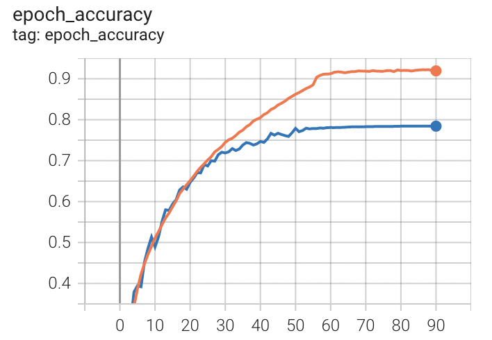
더이상 validation loss가 줄지 않을 때까지 돌려 91 epoch 동안 진행했다. 약 10시간이 소요됐다.
train loss는 0.7150, train accuracy는 0.9193으로 마무리 지었고, 최종 validation loss는 1.1215, validation accuracy는 0.7842였다.
이후 test dataset에 대해 평가한 결과 loss는 1.1369, accuracy는 0.7797이었다.

주황색이 train accuracy, 파란색이 validation accuracy이다.
코드 구현에 시행착오가 좀 있었다. Weight initialization에서, 처음에는 논문에 나온 그대로 mean=0, stddev=0.01인 random normal로 초기화했다. 그러나 아무리 기다려도, 몇번을 시도해도 loss가 일정 수준 이상으로 낮아지지 않았다. 물론 accuracy도 높아지지 않았다.
결국 weight initializer를 따로 설정하지 않고 학습을 시작하자 금방 원하는 결과가 나왔다.(위의 결과) Conv layer에 initializer를 설정하는 것 자체가 문제가 되는 모양인데, 원인을 좀 더 찾아봐야할 것 같다.
weight initializer는 상관이 없었다! 문제는 bias initializer였다. 그런데 여전히 알 수 없는 점은 왜 그런지이다. Bias를 두 개 이상 1로 설정하면 문제가 생기고, 그 중 하나를 약 0.8 미만으로 바꾸면 전혀 문제가 없다. 역시나 추가적인 고민이 필요하다.
optimizer 또한 논문처럼 SGD(momentum=0.9)를 사용했다. 이후 Adam optimizer를 사용해 다시 돌려봤는데, 약 4배 이상 빠르게 학습을 완료했다. 아무래도 웬만한 상황에선 Adam이 좋은 듯하다... 애초에 Adam은 AlexNet 논문의 시점으로부터 꽤 지난 2014년에 나왔으니 말이다.