이번 포스팅은 작년 데이터마이닝 수업을 통해 진행했던 과제를 간략하게 리뷰합니다.
What is the Data Mining?
데이터 마이닝이란 수많은 현실세계 데이터로부터 일종의 Nuggets 들을 뽑아내는 과정이라고 볼 수 있습니다.
기본적으로 데이터는 bulk 형태로 수집되지만, 우리가 어플리케이션 혹은 실생활에서 필요한 데이터는 유용한 Nuggets 형태의 구조입니다.
그렇기 때문에, 우리는 유용한 데이터를 얻기 위한 데이터 마이닝 과정을 진행합니다.
Data Mining Process
데이터 마이닝은 크게 3가지 과정으로 진행됩니다.
- 데이터 수집 (Data collection)
- 데이터 전처리 (Data Preprocessing)
- 데이터 훈련 (Data Training)
- 데이터 예측 (Data Prediction)
이번 포스팅에서는 데이터는 이미 수집 되어 있다는 가정 하에, 데이터 전처리, 데이터 훈련, 데이터 예측에 대해서 간략하게 소개합니다.
데이터 전처리 (Data Preprocessing)
실제 Raw 데이터들은 불필요한 데이터 존재, 결측값 존재, 정형화되지 않은 데이터 구조 형식 등으로 인해 데이터 훈련 및 데이터 분석을 하는데 있어서 사용하기 부적절합니다. 그렇기 때문에, 우리는 이 불안정한 데이터를 다듬어 일관성을 가질 수 있도록 해야합니다.
데이터 전처리 과정은 여러 과제들로 이루어져 있습니다. 데이터 일관성을 위해 데이터 전처리 과정은 training을 위한 데이터셋 뿐만 아니라, validation을 위한 데이터셋과, 예측하고자 하는 데이터셋에도 똑같이 적용해줍니다.
- Handle Missing Data
- Convert into Suitable Data Types
- Handle Duplicated Data
- Handle Irrelevant Attributes
- Perform Standardization
하지만, 데이터 전처리 과정을 진행하기 전에 데이터를 로드하여 데이터를 확인하는 작업이 필요합니다.
Data Loading
우리의 데이터는 sql형태로 주어져 있는데 이를 pandas data frame으로 불러와 데이터를 확인합니다.
train 데이터셋은 트레이닝을 위한 데이터이며, test 데이터셋은 class의 label을 예측하고자 하는 데이터입니다. 즉, classifiation 작업을 위해 class 컬럼의 라벨을 분류하는 것이 최종 목표입니다.
Training과 validation을 분리하는 작업은 이후 데이터 훈련 단계에서 진행합니다.
# Load the modules
import pandas as pd
import numpy as np
import sqlite3 as sql

from matplotlib import pyplot as plt

# connect to the database file.
db_file = "Assignment2022.sqlite"
con = sql.connect(db_file)

# Read sqlite query results into a pandas DataFrame
train_df = pd.read_sql_query("SELECT * from train", con)
test_df = pd.read_sql_query("SELECT * from test", con)

con.close()
데이터를 불러온 후, 데이터 구조 및 타입을 간략하게 확인합니다.
# check train data
train_df.describe()
train_df.info()<class 'pandas.core.frame.DataFrame'>
RangeIndex: 5000 entries, 0 to 4999
Data columns (total 31 columns):
# Column Non-Null Count Dtype
--- ------ -------------- -----
0 index 5000 non-null int64
1 Att00 5000 non-null float64
2 Att01 5000 non-null object
3 Att02 5000 non-null float64
4 Att03 5000 non-null float64
5 Att04 5000 non-null int64
6 Att05 5000 non-null float64
7 Att06 5000 non-null int64
8 Att07 5000 non-null float64
9 Att08 5000 non-null float64
10 Att09 5000 non-null float64
11 Att10 5000 non-null float64
12 Att11 5000 non-null object
13 Att12 5000 non-null object
14 Att13 5000 non-null float64
15 Att14 5000 non-null float64
16 Att15 5000 non-null float64
17 Att16 5000 non-null float64
18 Att17 5000 non-null int64
19 Att18 5000 non-null float64
20 Att19 5000 non-null float64
21 Att20 5000 non-null float64
22 Att21 5000 non-null float64
23 Att22 5000 non-null float64
24 Att24 5000 non-null float64
25 Att25 5000 non-null float64
26 Att26 5000 non-null int64
27 Att27 5000 non-null int64
28 Att28 5000 non-null float64
29 Att29 5000 non-null float64
30 class 5000 non-null float64
dtypes: float64(22), int64(6), object(3)
memory usage: 1.2+ MB
None또한, plot histogram을 통해서 numeric 데이터를 확인할 수 있습니다.
# we can plot a histogram of all the numeric data together.
train_df.hist(figsize=(20,20))
plt.show()
Handle Missing Data
결측치 관리 작업은 Missing data들을 제거하거나 적절한 방식으로 치환하여 데이터를 더 정교하게 만듭니다. 결측치를 제거하거나 치환하는 기준은 정해진 건 없지만, 이번 포스팅에서는 columns 내에 50% 이상 데이터가 N/A이면 제거, 20% 이하이면 mean value로 치환하는 작업을 진행 했습니다.
위의 train_df.describe()를 통해 우리는 count value가 데이터 사이즈와 동일하지 않은 column들을 결측치가 있는 데이터로 분류했습니다. 이를 통해 att50, att20 column이 결측치가 존재한다는 것을 확인할 수 있었고, 결측치비율을 계산하여 확인해줍니다.
# find which columns have greater 50% missing columns
def gt50_missing(df):
  df_rows = df.shape[0]
  target_cols = []
  for col in df.columns:
    if col == "class":
      continue
    missing = df[col].isna().sum()
    frac = missing / df_rows * 100
    if frac >= 50:
      target_cols.append(col)
  print(f"greater than 50% missing values in attribute: {target_cols}")
  return target_cols

# find which columns have less 20% missing columns
def lt20_missing(df):
  df_rows = df.shape[0]
  target_cols = []
  for col in df.columns:
    if col == "class":
      continue
    missing = df[col].isna().sum()
    frac = missing / df_rows * 100
    if 0 < frac < 20:
      target_cols.append(col)
  print(f'less than 20% missing values in attributes: {target_cols}')
return target_colsdrop을 통해 50%이상 결측치가 존재하는 컬럼은 삭제해주고, fillna를 통해, 20%미만 결측치가 존재하는 컬럼의 데이터들은 해당 컬럼의 mean 데이터로 치환해줍니다.
# find missing data and return its attributes
# drop the attributes
drop_cols = gt50_missing(train_df)
train_df.drop(columns=drop_cols, inplace=True)
test_df.drop(columns=drop_cols, inplace=True)

# find missing data and return its attributes
# replace the missing value to mean value
replace_cols = lt20_missing(train_df)
for col in replace_cols:
  train_mean = train_df[col].mean()
  train_df[col].fillna(train_mean, inplace=True)
  test_mean = test_df[col].mean()
  test_df[col].fillna(test_mean, inplace=True)
Select suitable Data Types
컴퓨터 혹은 머신은 문자보다는 숫자를 좀 더 잘 다룹니다. 그리고 scikit-learn (데이터 분석을 위한 라이브러리)은 string 형식의 데이터를 input으로 사용할 수 없습니다. 그렇기 때문에, string 형식의 데이터를 numeric 데이터 형식으로 인코딩 하는 작업이 필요합니다. 문자 데이터를 숫자 데이터로 치환하는데는 다양한 방법이 존재하지만, 이번 스터디에서는 가장 쉽고 널리 알려진 one-hot encoding을 사용했습니다.
우선 숫자 데이터 형식이 아닌, categorical columns을 확인합니다.
# detect categorical attributes
print(train_df.info())

# check the categorical data distribution.
category_cols = ['Att01', 'Att11', 'Att12']
for col in category_cols:
  print(f"train_df {col} distribution \n{train_df[col].value_counts()}")
  print(f"test_df {col} distribution \n{test_df[col].value_counts()}")
train_df Att01 distribution
OPHU 2109
UGRY 1846
EEVW 560
VMNM 427
OMJC 33
QDOP 24
HIWU 1
Name: Att01, dtype: int64예를 들면 Att01 컬럼에는 7가지 단어 집합 크기를 확인할 수 있습니다. 원핫 인코딩은 이 단어 집합(7)의 크기를 벡터의 차원으로 표현 후, 표현하고자 하는 단어의 인덱스를 1로, 이외 인덱스는 0으로 표현하여, 숫자형 데이터로 인코딩해주는 작업을 진행합니다.
from sklearn.preprocessing import OneHotEncoder

def one_hot_encoding(df, col):
  # value check in attribute
  # print(f"{col}:\n{df[col].value_counts()},")
  ohe = OneHotEncoder(sparse=False)
  cat = ohe.fit_transform(df[[col]])
  new_df = pd.DataFrame(cat, columns=[col+'_' + c for c in ohe.categories_[0]])
  return new_df

for col in category_cols:
  new_df = one_hot_encoding(train_df, col)
  train_df = pd.concat([train_df, new_df], axis=1)

for col in category_cols:
  new_df = one_hot_encoding(test_df, col)
  test_df = pd.concat([test_df, new_df], axis=1)

# drop the original categorical columns
train_df.drop(columns=category_cols, inplace=True)
test_df.drop(columns=category_cols, inplace=True)
원핫 인코딩을 해주고, 기존 categorical 컬럼은 제거해줍니다.
Handle duplicated Data
중복 데이터는 연산비용과 시간비용을 더 증폭시키는 안좋은 예입니다. 중복은 컬럼이 중복일 수도 있고, row별 데이터들이 중복으로 존재할 수도 있습니다. 이 두가지 케이스를 모두 확인하고, 중복을 제거해줍니다.
row 데이터 중복 확인
# detect duplicated instances
# no duplicated instances.
dups = train_df.duplicated()
print(dups.sum())

dups = test_df.duplicated()
print(dups.sum())
데이터 조회 후, sum()가 0이므로, 인스턴스별 중복은 없다는 것을 확인할 수 있습니다.
attributes 데이터 중복 확인
seaborn heatmap을 통해서 컬럼 중복을 확인합니다. 만약 컬럼에 normalization이 적용되어있다면, 값이 완전히 동일하지 않더라도 사실상 이는 동일한 컬럼입니다.
# detect duplicated attributes by heatmap
import seaborn as sns

# import seaborn as sns
def heatmap_covariance(df):
  fig, ax = plt.subplots(figsize=(30,30))         # Sample figsize in inches
  sns.heatmap(df.corr(), annot=True, linewidths=.5, ax=ax)

heatmap_covariance(train_df)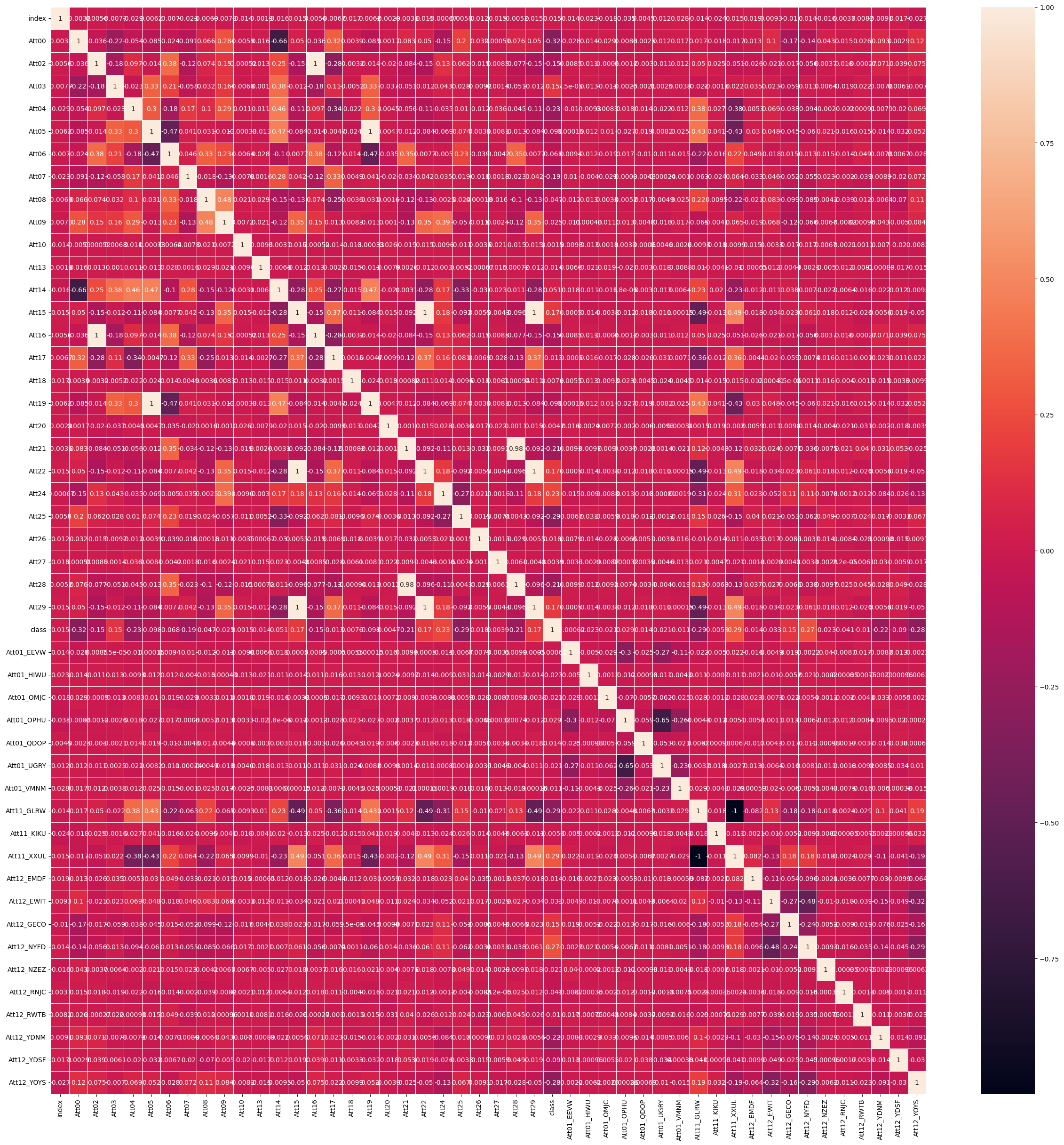
위의 heatmap을 통해 Att15, Att22, Att29, Att02, Att16, Att05, Att19가 중복으로 존재한다는 것을 확인 할 수 있습니다. 하나를 남기고 나머지 컬럼들은 제거해줍니다.
def drop_duplicated_columns(df):
  duplicated_columns = ['Att22', 'Att29', 'Att16', 'Att19']
  df.drop(columns=duplicated_columns, inplace=True)

drop_duplicated_columns(train_df)
drop_duplicated_columns(test_df)
Handle irrelevant attributes
각 attribute와 class 간의 상관관계를 분석하여 어느 것이 어느 정도 유용할지 파악합니다. 클래스와의 상관관계를 1% 미만인 attribute을 제거합니다.
heatmap_covariance(train_df)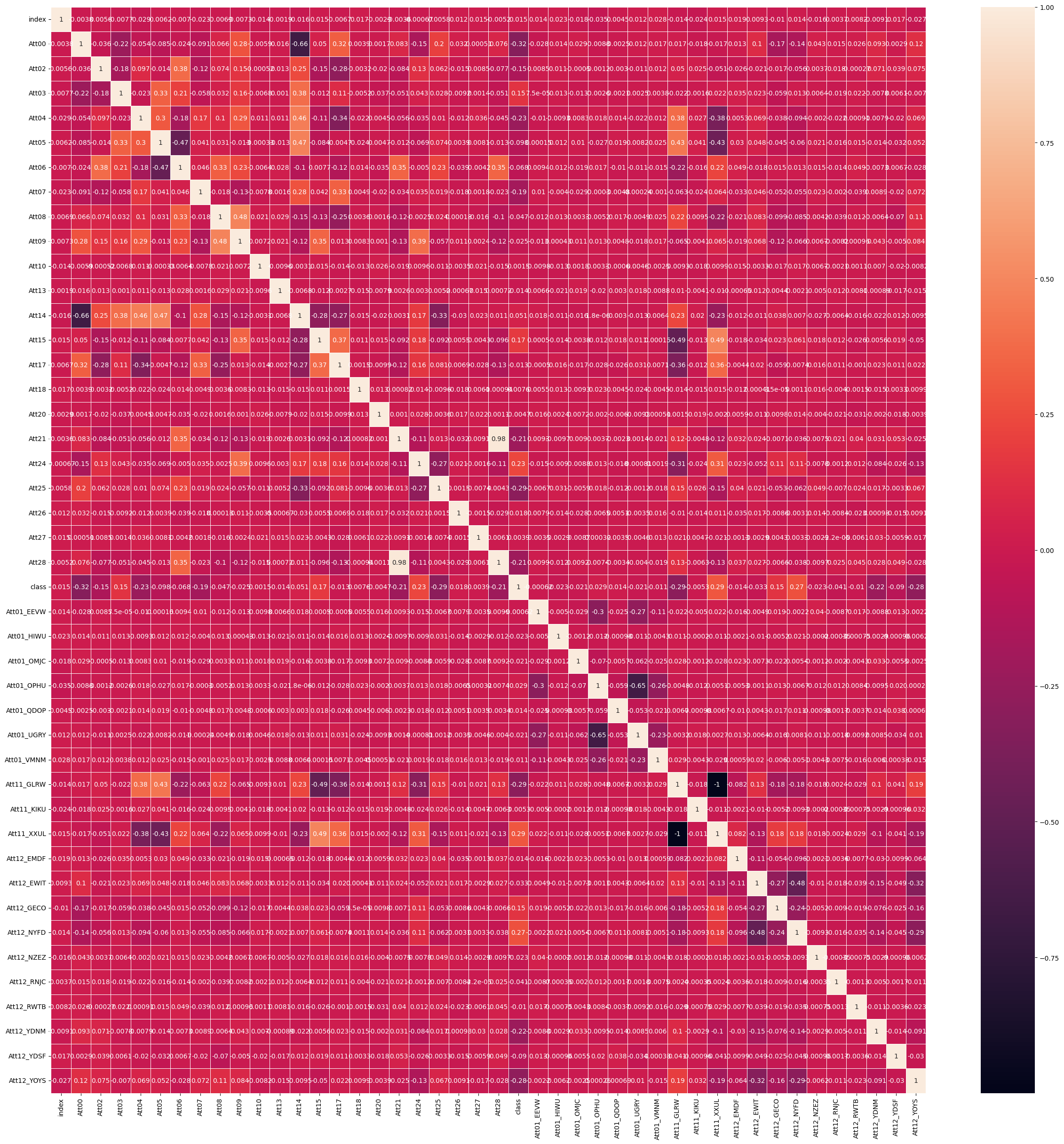
heatmap을 통해 Att10', 'Att18', 'Att20', 'Att27', 'Att01_EEVW', 'Att11_KIKU 컬럼이 1% 미만 상관관계를 가진다는 것을 확인할 수 있었습니다. 이 컬럼들을 제거해줍니다.
# drop the attributes with less 1% correlation to class
ls1_cols = ['Att10', 'Att18', 'Att20', 'Att27', 'Att01_EEVW', 'Att11_KIKU']
train_df.drop(columns=ls1_cols, inplace=True)
test_df.drop(columns=ls1_cols, inplace=True, errors='ignore')
Perform Standardization
모든 숫자 속성을 평균 0, 표준편차 1로 표준화하여 데이터 범위를 표준화합니다. sklearn에는 이를 수행하는 기능이 있습니다. index, class컬럼은 제외하고 표준화를 진행해줍니다
from sklearn.preprocessing import MinMaxScaler, StandardScaler

except_cols = ['index', 'class']

def standard(df):
  # choose all the numeric type attributes
  numeric_cols = df.select_dtypes(include='number').columns
  numeric_cols = numeric_cols.drop(except_cols, errors='ignore')

  # Create a standard scaler
  scaler = StandardScaler()
  # Determine the mean/std for each column and set up the scaler
  scaler.fit(df[numeric_cols])
  df[numeric_cols] = scaler.transform(df[numeric_cols])

standard(train_df)
standard(test_df)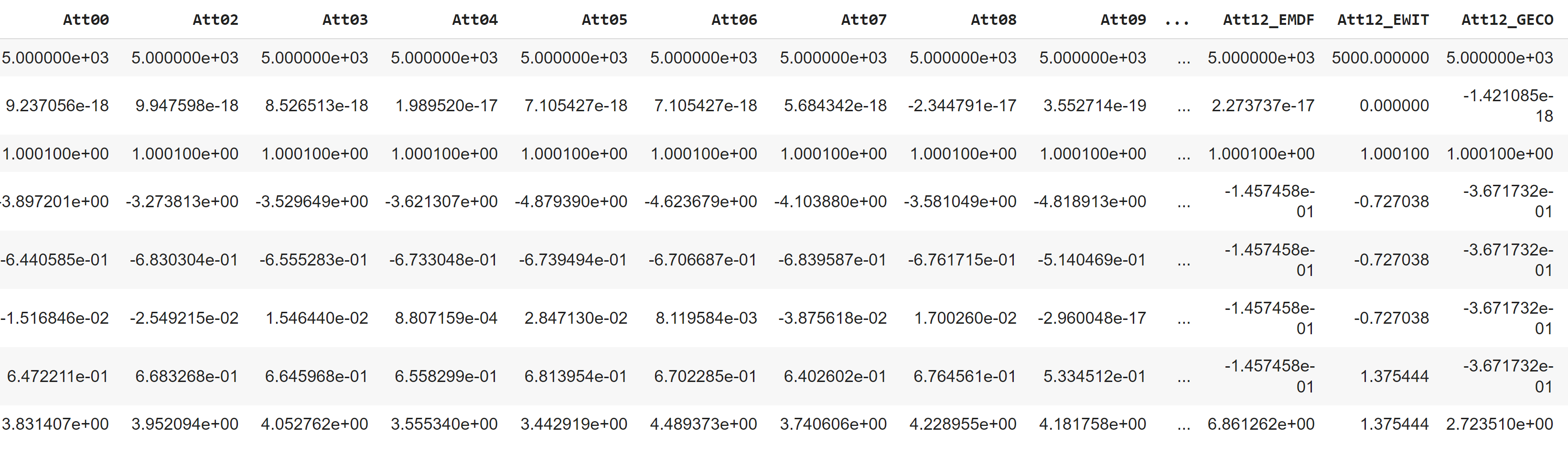
데이터 훈련 (Data Training)
테스트 데이터셋에서 누락된 레이블을 예측하기 위해 예측 모델을 선택, 교육 및 미세 조정합니다. k-NN, Naive Bayes, Decision Trees라는 세 가지 유형의 분류기를 거치게 됩니다.
이룰 위해 다음 과정을 진행합니다.
- 분류기를 위한 변수 설정
- 교차 검증 (Cross validation)을 위해 데이터를 분할하는 다양한 방법 살펴보기
- Model Training and Tuning
- K-NN Classifier
- Decision Tree Classifier
- Naive Classifier- Model 비교
분류기를 위한 변수 설정
데이터를 변수에 할당하여 모델에 최고의 성능을 제공하도록 하이퍼파라미터를 조정합니다. 여러 단계 끝에 'Att00', 'Att04', 'Att07', 'Att15', 'Att21', 'Att24', 'Att25', 'Att11_XXUL', 'Att12_NYFD', 'Att12_YDNM', 'Att12_YOYS' 컬럼들이 가장 좋은 성능의 모델을 만들어낸 다는 것을 확인했습니다.
model_cols = ['Att00', 'Att04', 'Att07', 'Att15', 'Att21', 'Att24', 'Att25', 'Att11_XXUL', 'Att12_NYFD', 'Att12_YDNM', 'Att12_YOYS']

X = train_df[model_cols].to_numpy()
y = train_df['class'].to_numpy()

X_train = train_df[model_cols].to_numpy()
y_train = train_df['class']

X_test = test_df[model_cols].to_numpy()
y_test = test_df['class']

# check the shape
X_train.shape, y_train.shape, X_test.shape, y_test.shape
((5000, 11), (5000,), (500, 11), (500,))validation체크를 위해 train 데이터셋와 validation 데이터셋을 9:1로 나눠줍니다.
from sklearn.model_selection import train_test_split

model_cols = ['Att00', 'Att04', 'Att07', 'Att15', 'Att21', 'Att24', 'Att25', 'Att11_XXUL', 'Att12_NYFD', 'Att12_YDNM', 'Att12_YOYS']

X = train_df[model_cols].to_numpy()
y = train_df['class'].to_numpy()

X_train, X_test, y_train, y_test = train_test_split(X, y,
                                                    test_size=0.1, # use a teste sieve of 25%
                                                    random_state=4) # this random state ensures that we get the same subset each time we call this cell
X_train.shape, y_train.shape, X_test.shape, y_test.shape
((4500, 11), (4500,), (500, 11), (500,))교차 검증 (Cross validation)을 위해 데이터를 분할하는 다양한 방법
우리의 Training 데이터셋에는 클래스 불균형 문제가 있습니다. 적은 수의 레이블이 지정된 클래스는 훈련 데이터에서 거의 발생하지 않으며 잘못 분류되는 경우가 많습니다. 교차 검증을 통해 모델/테스트 세트의 클래스 간 균형을 보장합니다.
이번 과제에서는 교차검증 메소드로, ShuffleSplit, KFold, 그리고 StratifiedKFold를 사용하여 비교했습니다.
# different ways to split data for cross validation
from sklearn import metrics
from sklearn.metrics import ConfusionMatrixDisplay
from sklearn.model_selection import StratifiedKFold, KFold, ShuffleSplit

# This is random sampling
ss = ShuffleSplit(n_splits=10, test_size=15, random_state=4) # 10 times of splits
# This is non-random sampling, we just break the data in to 10 contiguous sub-sets
kf = KFold(n_splits=10)
# Ensuring the balance between classes in the model/validate sets
# means we should use stratified sampling
skf = StratifiedKFold(n_splits=10)
# This cell sets up a nice visulisation that I found on the scikit-learn documentation page.
import matplotlib.pyplot as plt
from matplotlib.patches import Patch
cmap_data = plt.cm.Paired
cmap_cv = plt.cm.coolwarm
def plot_cv_indices(cv, X, y, group, ax, n_splits, lw=10):
"""
Create a sample plot for indices of a cross-validation object.
Adapted from https://scikit-learn.org/stable/auto_examples/model_selection/plot_cv_indices.html#define-a-function-to-visualize-cross-validation-behavior
Parameters
----------
cv: cross validation method
X : training data
y : data labels
group : group labels
ax : matplolib axes object
n_splits : number of splits
lw : line width for plotting
"""
# Generate the training/testing visualizations for each CV split
for ii, (tr, tt) in enumerate(cv.split(X=X, y=y, groups=group)):
# Fill in indices with the training/test groups
indices = np.array([np.nan] * len(X))
indices[tt] = 1
indices[tr] = 0
# Visualize the results
ax.scatter(range(len(indices)), [ii + .5] * len(indices),
c=indices, marker='_', lw=lw, cmap=cmap_cv,
vmin=-.2, vmax=1.2)
# Plot the data classes and groups at the end
ax.scatter(range(len(X)), [ii + 1.5] * len(X),
c=y, marker='_', lw=lw, cmap=cmap_data)
ax.scatter(range(len(X)), [ii + 2.5] * len(X),
c=group, marker='_', lw=lw, cmap=cmap_data)
# Formatting
yticklabels = list(range(n_splits)) + ['class', 'group']
ax.set(yticks=np.arange(n_splits+2) + .5, yticklabels=yticklabels,
xlabel='Sample index', ylabel="CV iteration",
ylim=[n_splits+2.2, -.2])
ax.set_title('{}'.format(type(cv).__name__), fontsize=15)
return ax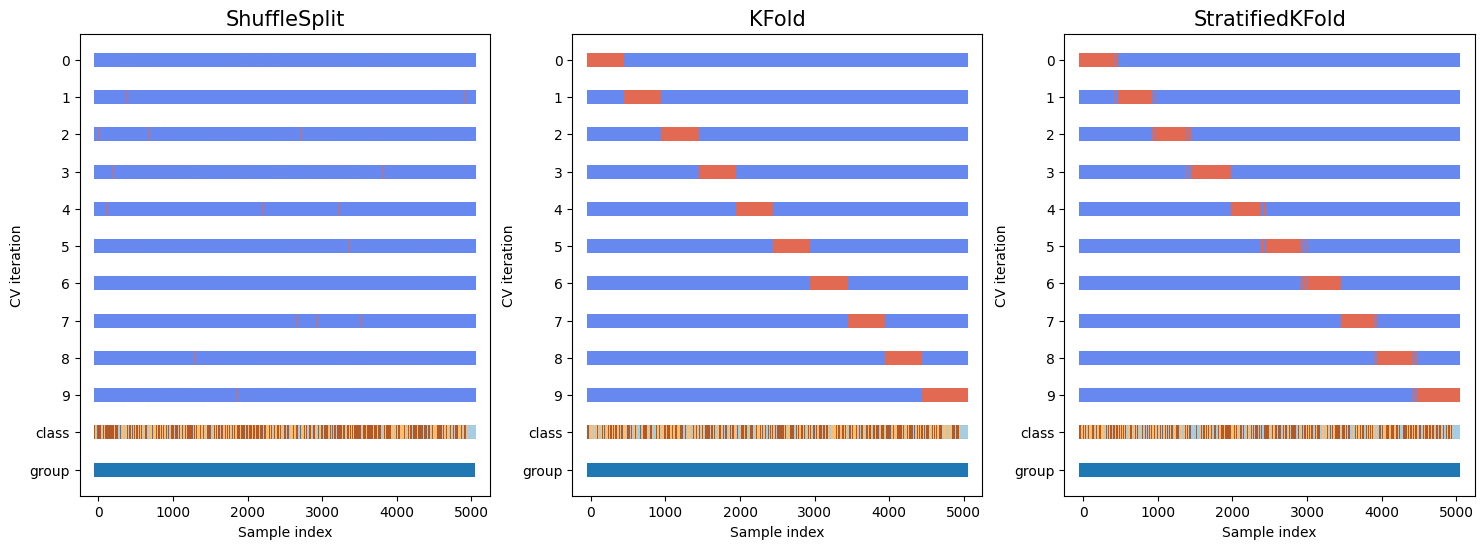
분류기 생성을 위해 class 레이블이 골고루 섞여있다는 것을 확인할 수 있습니다.
Model Training and Tuning
K-NN classifier
k-NN classifier를 사용하기 위해서 sklearn.neighbors.NearestNeighbors 라이브러리를 사용합니다. 다음 옵션을 사용하여 분류기를 훈련하고 오류율을 기록합니다.
weights = uniform or distancen_neighbors = 1 to 20
위의 여러 조합 중에서 정확도가 가장 높은 조합을 챔피언으로 선택하고, 테스트 데이터에 대한 예측 클래스와 실제 클래스를 비교하여 confusion matrix를 만듭니다.
from sklearn.neighbors import KNeighborsClassifier
from sklearn.model_selection import cross_val_score, GridSearchCV

#Create a dictionary of all the parameters we'll be iterating over
parameters = {'weights': ('uniform', 'distance'), # this should be the different weighting schemes
              'n_neighbors' : list(range(1, 20))}
# make a classifier object
knn = KNeighborsClassifier()
# create a GridSearchCV object to do the training with cross validation
gscv = GridSearchCV(estimator=knn,
                    param_grid=parameters,
                    cv=skf,  # the cross validation folding pattern
                    scoring='accuracy')
# now train our model
best_knn = gscv.fit(X_train, y_train)

best_knn.best_params_, best_knn.best_score_
({'n_neighbors': 12, 'weights': 'distance'}, 0.8055555555555556)Decision Tree classifier
Decision Tree classifier를 사용하기 위해서 sklearn.tree 라이브러리를 사용합니다. 다음 옵션을 사용하여 분류기를 훈련하고 오류율을 기록합니다.
분할(Splitting)을 위한 Gini Index와 Entropy, 그리고 2~20 사이의 min_samples_split 범위를 사용하여 분류기를 훈련합니다. 정확도 점수가 가장 높은 분류기를 최고의 분류기로 선택합니다.
from sklearn import tree

# Create a dictionary of all the parameters we'll be iterating over
parameters = {'criterion': ('gini','entropy'),  # this should be the different splitting criteria
              # 'min_samples_split':[3,10,15,20,25,40,50]} # this should be the different values for min_samples_split
              'min_samples_split': list(range(2,20))}
dtc = tree.DecisionTreeClassifier()
gscv = GridSearchCV(estimator=dtc,
                    param_grid=parameters,
                    cv=skf,
                    scoring='accuracy')
# now train our model
best_dtc = gscv.fit(X_train, y_train)

best_dtc.best_params_, best_dtc.best_score_
({'criterion': 'entropy', 'min_samples_split': 15}, 0.7066666666666667)plot 확인
fig, ax = plt.subplots(1,1, figsize=(30,30))
tree.plot_tree(best_dtc.best_estimator_,
               filled=True, # color the nodes based on class/purity
               ax=ax, fontsize=12)
plt.show()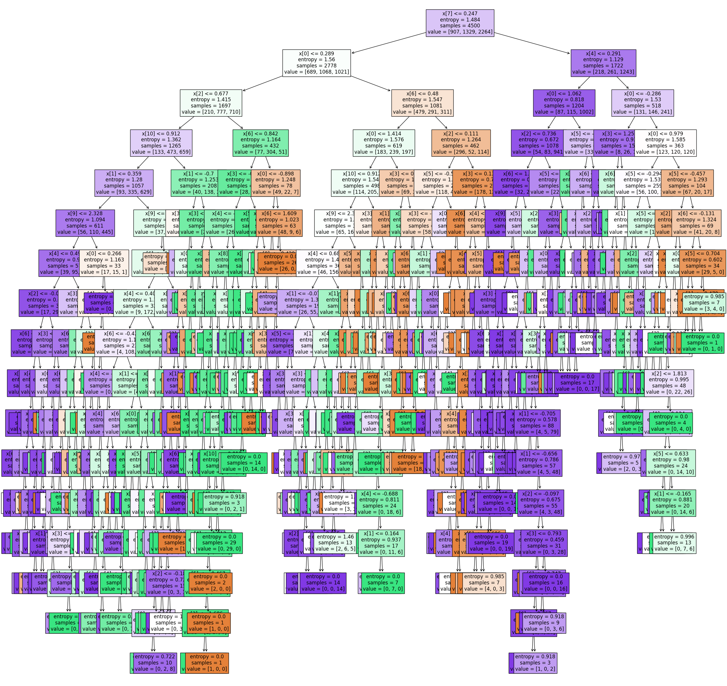
Naive-Bayes Classifier
Naive-Bayes Classifier를 사용하기 위해서 sklearn.naive_bayes 라이브러리를 사용합니다.
모든 훈련 데이터에 대해 분류기를 훈련시키고, 테스트 데이터의 클래스를 예측합니다.
마지막으로 Confusion Matrix를 확인합니다.
from sklearn import naive_bayes
# no parameters to adjust so no need to optimise, just train

nb = naive_bayes.GaussianNB()
nb.fit(X_train, y_train)
print(nb.score(X_train, y_train))

# print(nb.score(X_test, y_test))
# y_pred = nb.predict(X_test)
# accuracy = metrics.accuracy_score(y_train, y_pred)0.6782222222222222Model 비교
fig, ax = plt.subplots(1,3, figsize=(18, 6))

ConfusionMatrixDisplay.from_estimator(best_knn,
                                      X_test, y_test,
                                      display_labels=[0,1,2],
                                      ax=ax[0])

ConfusionMatrixDisplay.from_estimator(best_dtc,
                                      X_test, y_test,
                                      display_labels=[0,1,2],
                                      ax=ax[1])

ConfusionMatrixDisplay.from_estimator(nb,
                                      X_test, y_test,
                                      display_labels=[0,1,2],
                                      ax=ax[2])


plt.tight_layout()
plt.show()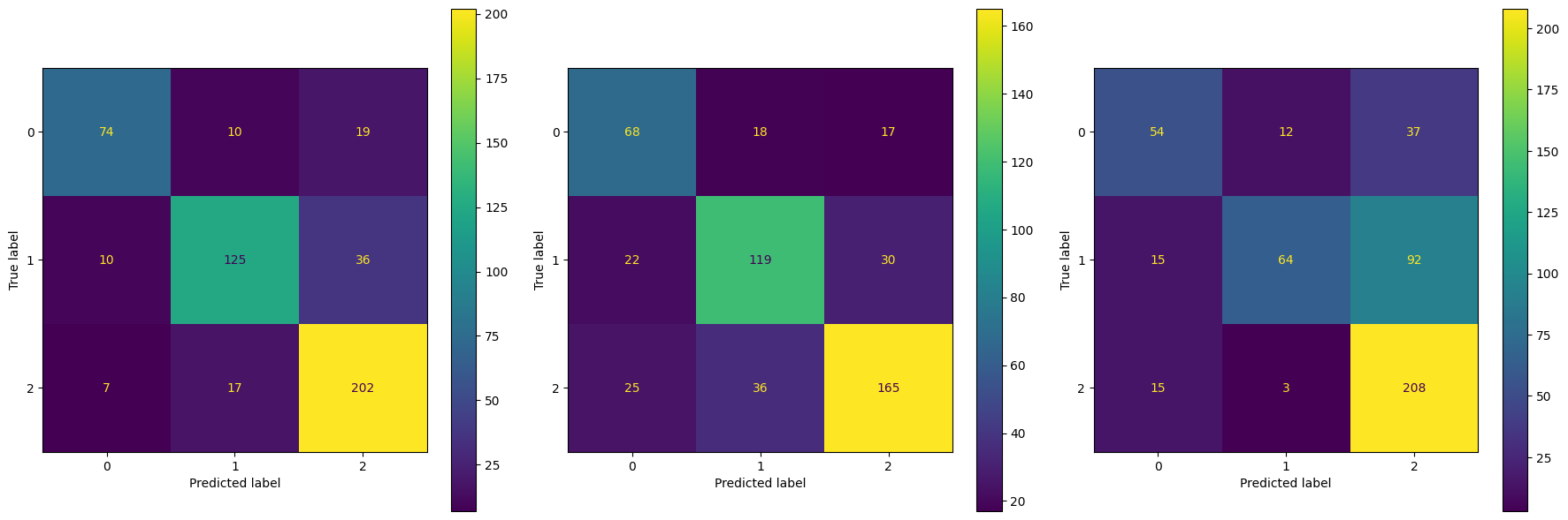
데이터 예측 (Data Prediction)
지금까지의 과정을 통해 가장 좋은 성능 모델은 K-NN과 Decision Trees라는 것을 알게 되었습니다.
모델을 훈련하고 테스트 데이터에서 누락된 레이블을 예측합니다. 그리고 ConfusionMatrixDisplay를 통해 시각적으로 정확성을 확인합니다.
X_train = train_df[model_cols].to_numpy()
y_train = train_df['class'].to_numpy()

X_pred = test_df[model_cols].to_numpy()
y_pred = test_df['class'].to_numpy() # not yet labeled

X_train.shape, y_train.shape, X_pred.shape, y_pred.shape
((5000, 11), (5000,), (500, 11), (500,))K-NN classifier 훈련 및 예측
# fit knn-model
classifier1 = KNeighborsClassifier(n_neighbors=k_neighbors, weights=k_weights)
classifier1.fit(X_train, y_train)

# new instances where we do not know the answer, which is the test data
# make a prediction
y_pred = classifier1.predict(X_pred)
y_pred_df = pd.DataFrame(y_pred, columns=['Predict1'])
test_df = pd.concat([test_df, y_pred_df], axis=1)
Decision Tree classifier 훈련 및 예측
# fit Decision Tree model with hyperparameter
classifier2 = tree.DecisionTreeClassifier(criterion='entropy', min_samples_split=15)
classifier2.fit(X_train, y_train)

# new instances where we do not know the answer, which is the test data
# make a prediction
y_pred = classifier2.predict(X_pred)
y_pred_df = pd.DataFrame(y_pred, columns=['Predict2'])
test_df = pd.concat([test_df, y_pred_df], axis=1)
분류결과 저장
final_df에 예측 결과를 저장합니다. prediction1은 knn을 통한 예측 결과, prediction2는 decision tree를 통한 예측 결과입니다.
final_df = pd.DataFrame(test_df[['index', 'Predict1', 'Predict2']], columns=['index', 'Predict1', 'Predict2'])
final_df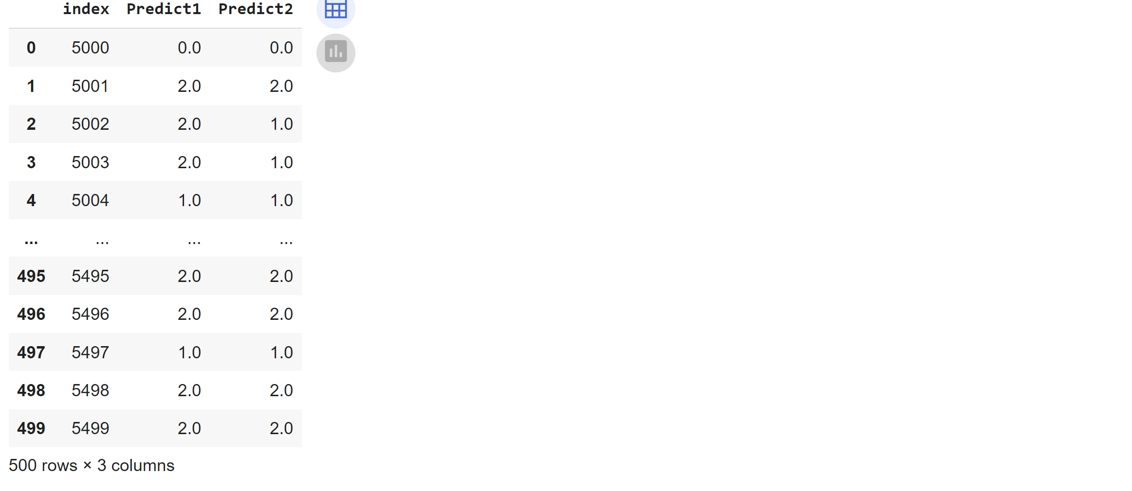
sqlite 파일로 저장
# make the result table
final_db_file = "Answers.sqlite"
make_db_con = sql.connect(final_db_file)
final_df.to_sql('answers', con=make_db_con, index=False)
make_db_con.close()
전체 소스는 링크를 통해 확인할 수 있습니다.