[Data Science] Frequent Pattern Mining (강의 1-4)
강의-데이터사이언스
0 Basic Concepts and a Road Map
1. Frequent Pattern Mining
☑️ FP: dataset에서 자주 나타나는 패턴.
❓ why) Finding inherent patterns in huge data
➰ ex) subsequences in DNA, substructures in GULF, co-purchased items in ITEM
2. Basic Concepts
- (just frequency)
- Probability that a trx contains .
- Minimum support: a threshold
- Conditional probability that a trx containing also contains .
- Minimum confidence: a threshold
Frequent Pattern
Association Rules
Closed & Max
▶️ use) FP가 너무 많은 경우 == useless patterns가 많은 경우
-
Closed Pattern
- same support인 FP들 중
- super pattern 無 인 FP
-
Max Pattern
- FP들 중
- super pattern 無인 FP
1 FP mining Method
❓ data가 매우 많으므로 reasonable time에 결과를 내기 위해서는 Scalable(==efficient == speed-up) 한 알고리즘이 필요하다.
0. Downward Closure Property of FP
FP의 특성으로, FP mining은 이 특성에 기반한다.
- FP이면, 그 subset도 FP이다.
- FP가 아니면, 그 superset도 FP가 아니다. (contraposition)
- (→ This can be used for pruning)
1. Apriori : Candidate Generation-and-Test Approach
☑️ Candidate Generation-and-Test Approach를 사용하는 FP mining Algorithm
❕ How
- 1st scan DB: get 1-itemset FP
- Repeat [k] (where k is length of itemset)
1) [k + 1]-Candidate를 생성한다. (self-joining [k]-FP -> pruning1)
2) 각 candidate가 FP인지 확인. (scan DB) (pruning2)
3) no FP || no Candidate 면 종료
Pseudo-code
C_k = candidate set of size k
L_k = frequent set of size k
L_1 = {freqiemt items};
for k = 1; L_k != {}; k++ {
	generate C_k+1
    for trx in database:
    	count C_k+1
	L_k+1 = elements over min_sup in C_k+1
}
return union of L_k
🥲 Pb)
- 多 DB scan (disk IO 에바징,,)
- 多 candidate, pruning에도 불구하고 (특히 k=1에서 많으면 k=2에서 반드시 많게 됨)
- 多 workload (특히 candidate의 support counting)
ex) 100개 item -> 100 scans, candidates
sol) general ideas
- DB scan ↓
- candidate 수 ↓
- candidate support counting을 고도화
Sol) DIC, Partition, Sampling, DHP
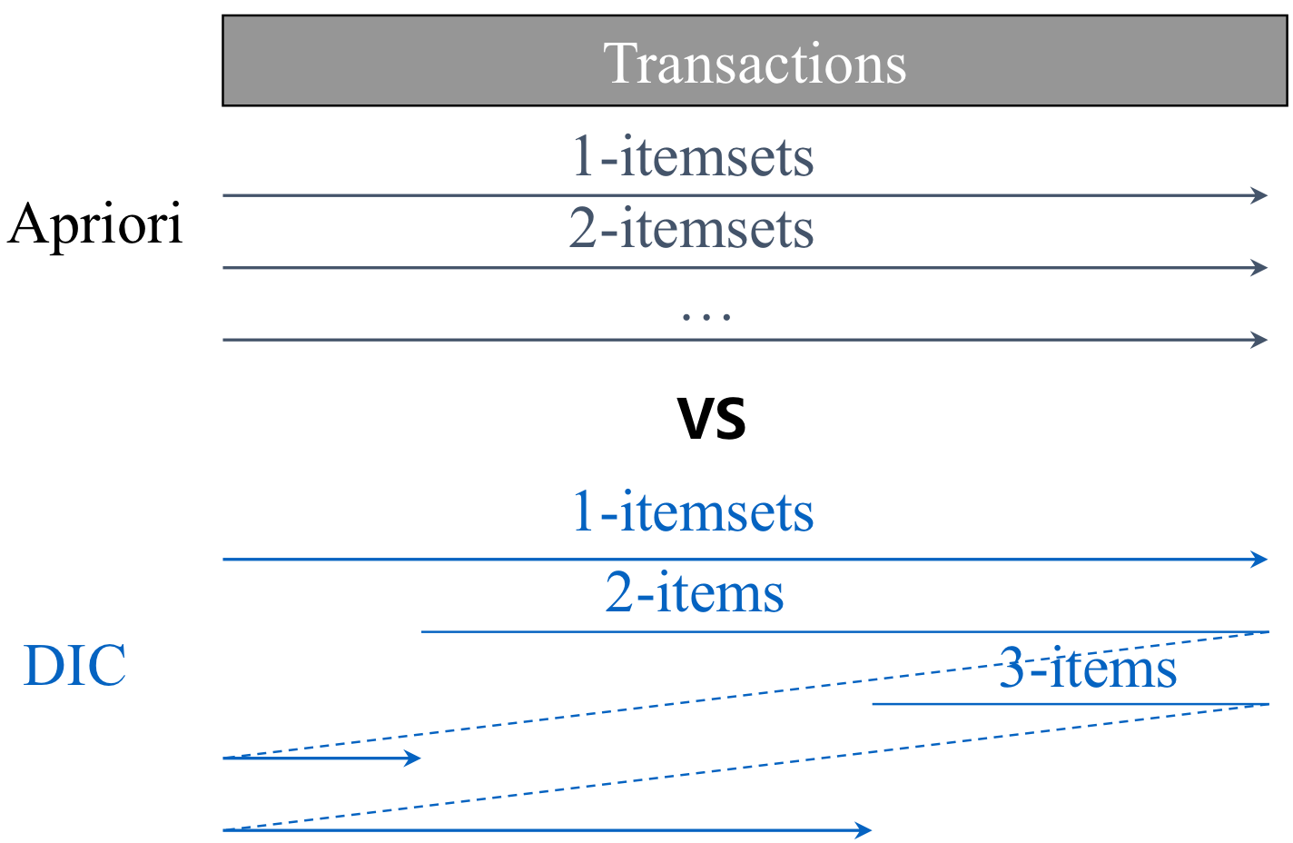
1. DIC (Dynamic)
(Dynamic Itemset Counting)
☑️ candidate-generation-and-test를 동적으로 수행하는 알고리즘
-> [k]에서 k-candidate만을 counting하지 않고, k+1-candidate도 생성하여, 생선한 즉시 support counting을 시작한다.
👍🏻 gd) DB scan ↓
2. Partition (2 scan)
☑️ DB을 분할하여 각 partition에서 apriori를 수행하는 알고리즘
👍🏻 gd) 2 DB scan
👍🏻 gd) guarantee ALL FP (❓global FP는 at least one partition에서 local FP가 된다.)
❕ how) algorithm
1) DB를 main memory에 fit하게 k개로 나눈다.
2) local FP를 구한다. → local_min_sup = min_sup/k
3) global FP인지 테스트한다.
3. Sampling
☑️ DB에서 random smapling으로 SDB(Sample DB)를 만들어 Apriori를 수행하는 알고리즘
👍🏻 gd) DB scan ↓, candidate 수 ↓
🥲 pb) not global FP 可, FP missed 可
-> sol) 2 more scan
1. Verify FP and its negative borders (NB: S에는 없으나, S에 모든 subset들이 있는 경우 + single items)
2. NB
4. DHP (Hashing)
(Direct Hashing and Pruning)
candidate를 해싱을 이용하여 pruning하며 Apriori를 수행하는 알고리즘
👍🏻 gd) candidate 수 ↓
how)
1. Hashing: [k] 각 trx에서 k+1-candidate를 만들고 해싱한다.
2. Pruning: 해싱 테이블에 기반하여 candidate를 pruning하고 test
2. FP-growth
☑️ Apriori의 main bottleneck인 candidate-genration-and-test 과정 없이 FP를 찾기 위해 고안된 FP mining 기법
👍🏻 gd) candidate generation & test 가 없다
👍🏻 gd) FP-tree가 compressed DB의 역할을 하여 데이터를 메모리 내에서 다룰 수 있다. -> 2 scan of DB (FP-tree 만드는 과정에서 2번)
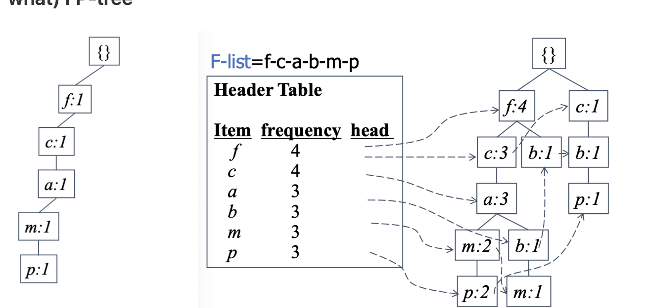
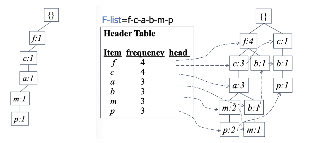
1) FP-tree
☑️ FP-Growth에서 사용되는 자료구조이다.
- 3 자료구조 : F-list, Header Table, FP-tree
👍🏻 gd) Completeness : lossless info.를 가진다.
👍🏻 gd) Compactness : infrequent item이 없어서 compact하므로 매모리에 올라올 수 있다, freq 할수록 더 위에 있으므로 공유될 가능성 ↑
how) to make
- Scan DB, find frequent 1-itemsets
- Make F-list: Sort 1-FP in frequencey descending order(strict order가 있어야 함)
- Scan DB,
1) F-list를 사용하여 각 trx를 배열한다.
2) Construct FP-tree
2) How to find FP: divide-and-conquer
- Divide → Target FP를 disjoint subset으로 partitioning
- Conquer → each parition에서 F-list를 사용하여 conditional patt-base와 conditional FP-tree를 생성한다.
- conditional FP-tree가 single path, empty 멈춘다.
- branch가 있다면 recursion
3) cf) FP-Growth vs. Apriori
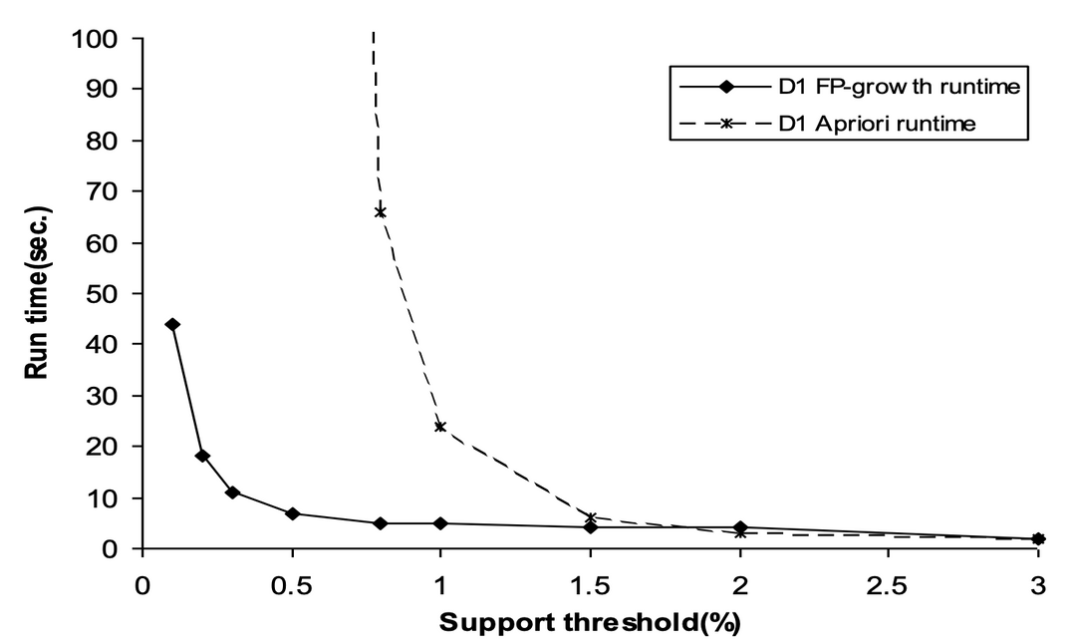
- 大 min_sup → Apriori에서 생성&테스트 candidate의 수가 절대적으로 적어지므로 두 알고리즘의 차이가 거의 없다.
- 小 min_sup → FP-Growth에서는 candidate generation and test가 없으므로 압도적으로 성능이 좋다.
3. Max Miner
Mining Max Patterns
FP X
only max-pattern O
- 1-FP를 찾고 ascending order로 정렬한다.
- 2-FP부터 potential max-pattern을 찾는다. by set-enumeration tree
👍🏻 gd) 2-FP부터 potential max-patt.을 검사하면 이후 단계에서 candidate의 수가 줄어든다. (BCDE O → BCD, BDE, CDE 체크할 필요 X)
4. CLOSET
Mining Closed Patterns
FP-growth 중에 closed pattern을 찾을 수 있다.
m-conditional base에서 closed patt. 찾기
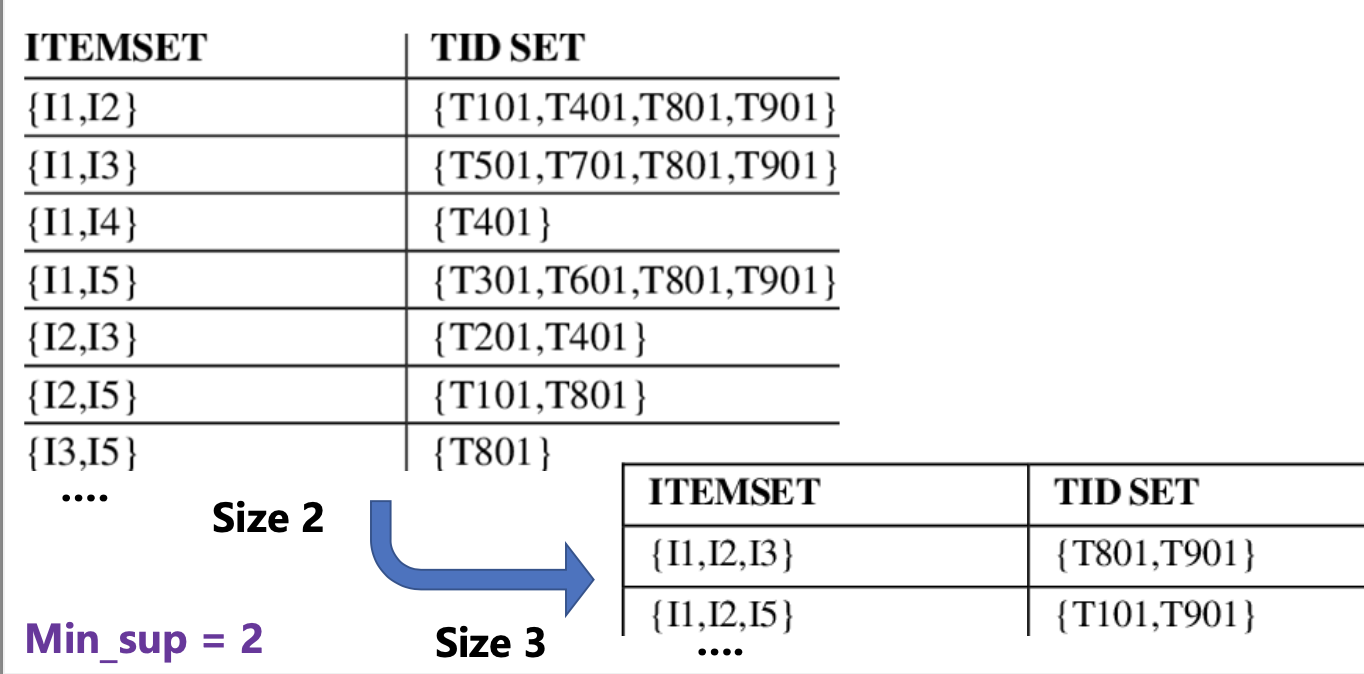
5. CHARM
(Closed itemset based High Utility Rare Itemset Mining)
Vertical format 을 활용하여 FP를 찾는다.
👍🏻 gd) 교집합 operation으로 candidate를 얻을 수 있다.
👍🏻 gd) length가 frequency이다
- 1 FP itemset들을 vertical format으로 바꾼다.
- k + 1 size의 FP itemset을 찾는다. (교집합 + APriori property)
2 Association Rules
1. Multi-Level Association Rules
Item은 hierarchies를 가지므로 flexible min_sup을 설정한다.
ex) milk (10%) 매일우유(6%), 서울우유(4%)
❓ 다른 계층에 같은 minimum support를 적용하는 것은 unfair
goal) 다른 계층의 같은 아이템들이 최대한 같게 FP에 포함되도록 (milk가 FP면 매일우유&서울우유도 FP가 되도록)
Redundancy Filtering
ancestor rule
descendant rule
descendant support가 ancester support에 의해 expected value이면 redundant
2. Multi-Dimensional Association
- single-dim. -> buy(milk) -> buy(bread)
- multi-dim.
- inter-dim. -> age(19-25) ^ occupation(student) -> buy(coke)
- hybrid-dim. -> age(19-25) ^ buy(popcorn) -> buy(coke)
3. Quantitative Association
Attribute(Feature) 유형
- Categorical -> finte, order X
- Quantitative -> numeric, order O
numeric feature로부터 연관 규칙 찾기
- Design the format of association rule.
- Discretize the features
- Make a grid
- Calculate each cell
*adjacent cell이면 합칠 (cluster) 수 있다.
3 From Association Mining to Correlation Analysis
ex) play basketball -> eat cereal (0.4, 0.67)
🥲 pb) meaningful해 보이지만 사실 eat cereal은 75%이다.
-> sol) interstingness measure : lift
- -> positive correlation
- -> independent
- -> negative correlation